Griffiths D.F., Higham D.J. Numerical Methods for Ordinary Differential Equations: Initial Value Problems

Подождите немного. Документ загружается.

186 13. Modiﬁed Equations

3. Should the values of u and v be required at time t = t

n+1

= u

−

n+1

Thus, v is computed at integer nodes and u at half-integer nodes.

For the purposes of analysis, all half-integer values are eliminated from

(13.18), so the update from u

, v

to u

n+1

, v

n+1

may be written as



n+1







+ h



−v



−









. (13.22)

Before embarking on the construction of modiﬁed equations we check the

LTE of the method. The original ODE system is expressed in matrix-vector

form as

(t) = Au(t), A =



0 −1

1 0



and we observe that A

= −I, A

= −A so that

(t) = Au

(t) = A

u(t) = −u(t), u

000

(t) = −u

(t) = −Au(t).

The Taylor expansion

u(t + h) = u(t) + hu

(t) +

000

(t) + O(h

)

therefore becomes

u(t + h) =



I + hA −

I −



u(t) + O(h

Equation (13.22) can be written in matrix-vector form as

n+1



I + hA −

I +



0 1

0 0





so, under the localizing assumption u

= u(t

), we have

u(t

n+1

) − u

n+1

= O(h

showing that the St¨ormer–Verlet method is consistent of order 2.

We next seek a matrix B so that the numerical solution is consistent of

order three with the modiﬁed system

(t) = (A + h

B)x(t). (13.23)

It follows by successive diﬀerentiation that

(t) = (A + h

B)x

(t) = (A + h

x(t) + O(h

)

= A

x(t) + O(h

) = −x(t) + O(h

)

13.3 A Two-Step Method 187

and x

000

(t) = −Ax(t) + O(h

). Using these in the Taylor expansion of x(t + h)

we ﬁnd

x(t + h) = x(t) + hx

(t) +

000

(t) + O(h

)

= x(t) + h(A + h

B)x(t)

−

− x(t) −

Ax(t) + O(h

)

I + hA −

I − h

(

A + B)

x(t) + O(h

Now, under the localizing assumption that u

= x(t

), we ﬁnd

x(t

n+1

) − u

n+1

= h



−

A + B −



0 1

0 0





x(t

) + O(h

The right-hand side will be of fourth order if

B =

A +



0 1

0 0





0 −1

2 0



The St¨ormer–Verlet method is, therefore, consistent of order three with the

modiﬁed system (13.23). It then follows (see Exercise 13.10) that the compo-

nents of x(t) lie on the ellipse

(1 +

(t) + (1 +

(t) = constant (13.24)

and, from the initial conditions, the constant = 1 +

. This is shown as a

dashed curve in Figure 13.3 (right) when h = 1/3 and is virtually indistinguish-

able from the circle on which the exact solution u(t) lies.

It was shown in Example 7.6 that the solutions of the trapezoidal rule

lie on precisely the same circle as the exact solution of the IVP. This would

appear to give it an advantage over the symplectic Euler method (13.18) and

the St¨ormer–Verlet method (13.21). However, counting against the trapezoidal

rule are the facts that (a) it is implicit and, therefore computationally expensive

in a nonlinear context, and (b) the exact “conservation of energy” property does

not generalize to nonlinear problems as it does for the other methods.

13.3 A Two-Step Method

The e xamples thus far have sought to ﬁnd a modiﬁed equation with which the

method has a higher order of consistency than with the original ODE. Our ﬁnal

example has a diﬀerent nature and shows that a method applied to a scalar

problem may also be a consistent approximation of a system.

188 13. Modiﬁed Equations

Example 13.6 (The Mid-Point Rule)

Derive a modiﬁed system of equations that can be used to explain the behaviour

of the mid-point rule (see Example 6.12) when it is used to solve the IVP

(t) = u(t) − u

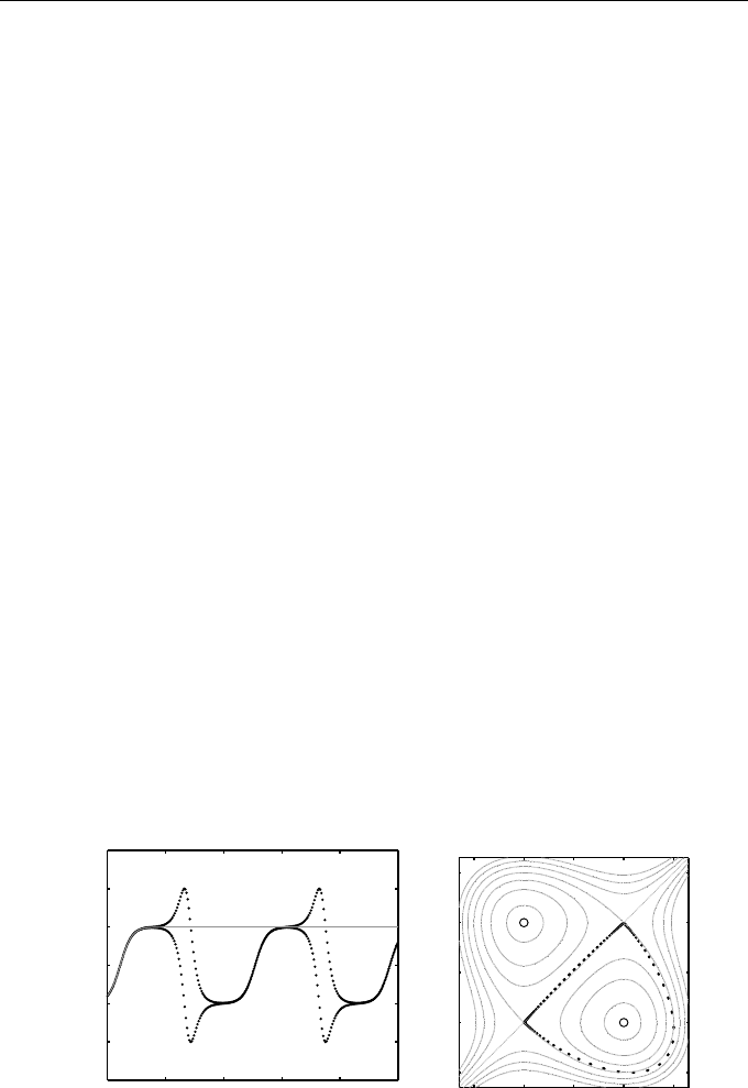
(t), u(0) = 0.1. The numerical solution with h = 0.1 is shown

in Figure 13.4 (left) and is seen to have periodic bursts of activity while the

exact solution is eﬀectively constant for t > 5.

The mid-point rule applied to the given ODE leads to the nonlinear diﬀer-

ence equation

n+2

− u

= 2hu

n+1

(1 − u

n+1

) (13.25)

with u

= 0.1 and we assume that the second initial condition is obtained via

Euler’s method:

= u

+ hu

(1 − u

We observe in Figure 13.4 (left) that the numerical solution (dots) is indis-

tinguishable from the exact solution (solid curve) up until about t = 5, after

which consecutive values of u

oscillate around the steady state u = 1. This

suggests that we treat the even- and odd-numbered values of u

diﬀerently. We

shall suppose that, u

≈ x(t

) for even values of n and that u

≈ y(t

) for odd

values of n, where the smooth functions x(t) and y(t) will be the solutions of

a (yet to be determined) modiﬁed system of ODEs.

The LTE will be diﬀerent depending on the parity of n:

n+2

(

x(t

n+2

) − x(t

) − 2hy(t

n+1

)



1 − y(t

n+1

)



, when n is even,

y(t

n+2

) − y(t

) − 2hx(t

n+1

)



1 − x(t

n+1

)



, when n is odd,

(13.26)

0 10 20 30 40 50

−1

−0.5

0.5

1.5

−0.5 0 0.5 1 1.5

−0.5

0.5

1.5

Fig. 13.4 Left: numerical solutions for Example 13.6 with h = 0.1 (dots) and

the exact solution u(t) (solid curve). Right: the numerical solution (dots) is

seen to lie on one of the family (13.28) of ellipses in phase space

13.3 A Two-Step Method 189

and Taylor expansion

leads to

n+2

(



n+1

) − y(t

n+1

)



1 − y(t

n+1

)



+ O(h

), when n is even,



n+1

) − x(t

n+1

)



1 − x(t

n+1

)



+ O(h

), when n is odd.

This suggests that the method, which is a one-step map from (u

, u

n+1

) to

n+1

, u

n+2

), is consistent of order 2 with the system

(t) = y(t) − y

(t)

(t) = x(t) − x

(t)

)

. (13.27)

In contrast to the previous examples this system does not have h-dependent

coeﬃcients. Since

(t)

we deduce that y, regarded as a function of x, satisﬁes the separable diﬀerential

equation

(y(t) − y

(t))

= x(t) − x

(t).

This can be integrated to give (following factorization)

(x − y)



x +

y −

+ xy + y

)



= constant. (13.28)

These curves are shown in Figure 13.4 (right) with values −0.15, −0.1, . . . , 0.15

for the constant. Superimp ose d are the points (u

, u

2m−1

) showing even- ver-

sus odd-numbered values of the solution sequence. The dots leading directly

from the origin O to the point marked A(1, 1) correspond to the smooth part

of the trajectory up to about t = 5. On OA we have x = y, which implies

that x = y = u, and so even- and odd-numbered points both approximate the

original solution u(t).

When the solution approaches the steady state we can substitute u(t) =

1 − εv(t) into u

(t) = u(t) − u

(t) to give v

(t) = −v(t) + εv

(t). When ε is

small, u(t) is close to 1 and the linearized equation

(t) = −v(t) indicates

that the solution is attracted to v = 0, that is u = 1, exponentially in time.

However, it was shown in Example 6.12 that the mid-point rule cannot be

absolutely stable for any h > 0. It is this loss of (weak) stability that causes

the oscillatory b e haviour—corresponding to a trajectory moving in a closed

semi-elliptic path in the phase plane. The long-term behaviour of the system

(13.27) is the subject of Exercise 12.1.

It is more eﬃcient here to Taylor expand each of the quantities x(t

n+2

), x(t

y(t

n+2

), y(t

) about t = t

n+1

because this avoids having to expand the nonlinear

terms.

See Section 12.1 on Long Term Dynamics.

190 13. Modiﬁed Equations

How can this behaviour be rec onciled with the fact that, because the mid-

point rule is zero-stable and a consistent method of order 2 to the original

ODE, its solutions must converge to u(t), the solution of u

(t) = u(t) − u

(t),

u(0) = 0.1? In the phase plane it takes an inﬁnite time for the exact solution

of the ODEs to reach the point A and convergence of a numerical method is

only guaranteed for ﬁnite time intervals [0, t

]. Moreover, as h → 0, the time at

which the instability sets in tends to inﬁnity and so the motion on any interval

[0, t

] is ultimately free of oscillations.

13.4 Postscript

In cases where the modiﬁed equations are diﬀerential equations with h-dependent

coeﬃcients they should tend towards the original diﬀerential equations as

h → 0. This provides a basic check on derived modiﬁed equations. See the

article by Griﬃths and Sanz-Serna [24] for further examples of modiﬁed equa-

tions for both ordinary and partial diﬀerential equations in a relatively simple

setting.

Modiﬁed equations are related to the idea of “backward error analysis”

in linear algebra that was developed around 1950 (see N.J. Higham [36, Sec-

tion 1.5]). The motivating idea is that instead of regarding our computed values

as an approximate solution to the given problem, we may regard them as an

exact solution to a nearby problem. We may then try to quantify the concept

of “nearby” and study whether the nearby problem inherits properties of the

given problem. In our context, the nearby problem arises by adding small terms

to the right-hand side of the ODE. An alternative would be to allow the initial

conditions to be perturbed, which leads to the concept of shadowing. This has

been extensively studied in the context of dynamical systems (see, for example,

Chow and Vleck [8]).

EXERCISES

13.1.

For Example 13.1, amend the proof of Theorem 2.4 to prove that

ˆe

= O(h

) (Hint: it is only necessary to take account of the fact

that |

| ≤ Ch

13.2.

Show that the LTE (13.3) is of order O(h

) when y(t) is the solution

of the alternative modiﬁed Equation (13.8). Hence, conclude that x

is a second-order approximation to y(t

). Show that the arguments

based on (13.6) ab out the overdamping eﬀ ec ts of Euler’s method

Exercises 191

could also be deduced from (13.8).

13.3.

Show that the LTE (13.3) is of order O(h

) when y(t) is the solution

of the modiﬁed equation y

(t) = µy(t), where

µ = λ



1 −

λh +



Hence, conclude that x

is a third-order approximation to y(t

13.4.

Consider the backward Euler method (1 − λh)x

n+1

= x

applied

to the ODE x

(t) = λx(t). Show that the LTE is given by

n+1

= y(t

+ h) − (1 − λh)

−1

y(t

)

and is of order O(h

) when y(t) satisﬁes the second-order ODE

(t) = λ(1 +

λh)y(t).

Deduce that |y(t)| > |x(t)| for t > 0 when 0 < 1 +

λh < 1 and

y(0) = x(0).

13.5.

Consider the backward Euler method x

n+1

= x

+ hf

n+1

applied

to the ODE x

(t) = f (x(t)). By writing x

n+1

= x

+ δ

, show that

f(x

n+1

) = f (x

) + h

)δ

+ O(h

Use this, together with the expansion (13.4) and the localizing as-

sumption, to deduce the modiﬁed equation

(t) =



1 +

(y(t))



f(y(t)). (13.29)

13.6.

Show that y

(t) = A(I −

hA)y(t) is a modiﬁed equation for Euler’s

method applied to the linear syste m of ODEs x

(t) = Ax(t), where

x, y ∈ R

and A is an m × m matrix.

Identify an appropriate matrix A for the ODEs in Example 13.3 and

verify that the “modiﬁed matrix” in (13.16) is

A = A(I −

hA).

An alternative way of ﬁnding suitable values of µ is to substitute y(t) = e

µt

into

(13.3) to give

n+1

= e

µt

µh

− 1 − λh

. Hence,

n+1

= O(h

p+1

) if µ is chosen so

that e

µh

= 1 + λh + O(h

p+1

). Thus, µ can be obtained by truncating the Maclaurin

series expansion of

µ =

log(1 + λh) = λ −

h +

+ ··· + (−1)

p+1

+ ··· .

192 13. Modiﬁed Equations

13.7.

???

Use the modiﬁed system derived in the previous ques tion to discuss

the behaviour of Euler’s method applied to x

(t) = Ax(t), when

x(t

) is an eigenvector of A, in the cases where the matrix A is (a)

positive deﬁnite, (b) negative deﬁnite, and (c) skew-symmetric.

13.8.

Use the identity



(t) + y

(t)



= 2x(t)x

(t) + 2y(t)y

(t)

together with the ODEs (13.15) to prove that



(t) + y

(t)



= h



(t) + y

(t)



which is a ﬁrst-order constant-coeﬃcient linear diﬀerential equation

in the dependent variable w(t) = x

(t) + y

(t). Hence, prove that

x(t) and y(t) satisfy Equation (13.17).

13.9.

Complete the details leading up to (13.19).

Show that



(t) − hx(t)y(t) + y

(t)



= 0

and, hence, deduce that Equation (13.20) holds.

13.10.

Deduce that the solutions of the modiﬁed system derived in Exam-

ple 13.5 lie on the family of ellipses (13.24).

13.11.

???

Show that the nonlinear oscillator u

(t) + f(u) = 0 (cf. Exer-

cise 7.6) is equivalent to the ﬁrst-order system

(t) = −v(t), v

(t) = f (u(t)). (13.30)

Supp ose that F (u) is such that f (u) =

dF (u)

. Show that the solu-

tions of this system satisfy



2F (u(t)) + v

(t)



= 0

and, therefore, lie on the family of curves v

(t)+2F (u(t)) = constant.

The system (13.30) may be solved numerically by a generalization

of the method in Example 13.4:

n+1

= u

− hv

, v

n+1

= v

+ hf (u

n+1

), n = 0, 1, . . . ,

with u

= 1 and v

= 0. Derive the modiﬁed system

(t) = −y(t) +

hf(x(t))

(t) = f(x(t)) −

(x(t))y(t)







Exercises 193

Deduce that



2F (x(t)) − hf(x(t))y(t) + y

(t)



= 0

and hence that solutions lie on the family of curves

2F (x(t)) − hf(x(t))y(t) + y

(t) = constant

in the x-y phase plane. Verify that these results coincide with those

of Example 13.4 when f(u) = u.

13.12.

???

It follows from Exercise 11.3 that the TS(1) method of Exam-

ple 11.2 applied to the IVPx

(t) = −λx(t), x(0) = 1, leads to

n+1

= (1 − h

λ)x

, t

n+1

= t

+ h



2 tol



1/2

, t

= 0, x

= 1,

(13.31)

on the assumption that no steps are rejected. Suppose that (t

, x

)

denotes an approximation to a point on the parameterized curve

(t(s), x(s)) at s = s

, where s

= n∆s and ∆s =

√

2tol is a constant

step size in s. Assuming that λ > 0, show that the equations (13.31)

are a consistent approximation of the IVP

x(s) = −λg(s)x(s),

t(s) = g(s),

with x(0) = 1, t(0) = 0, and g(s) = 1/(λ

x(s)).

Solve these ODEs for x(s) and t(s) and verify that the expected

solution is obtained when the parameter s is eliminated. Show that

x(s) = 0 for s = 2 regardless of the value of λ. Deduce that the

numerical solution x

is expected to reach the ﬁxed point x = 0

in approximately

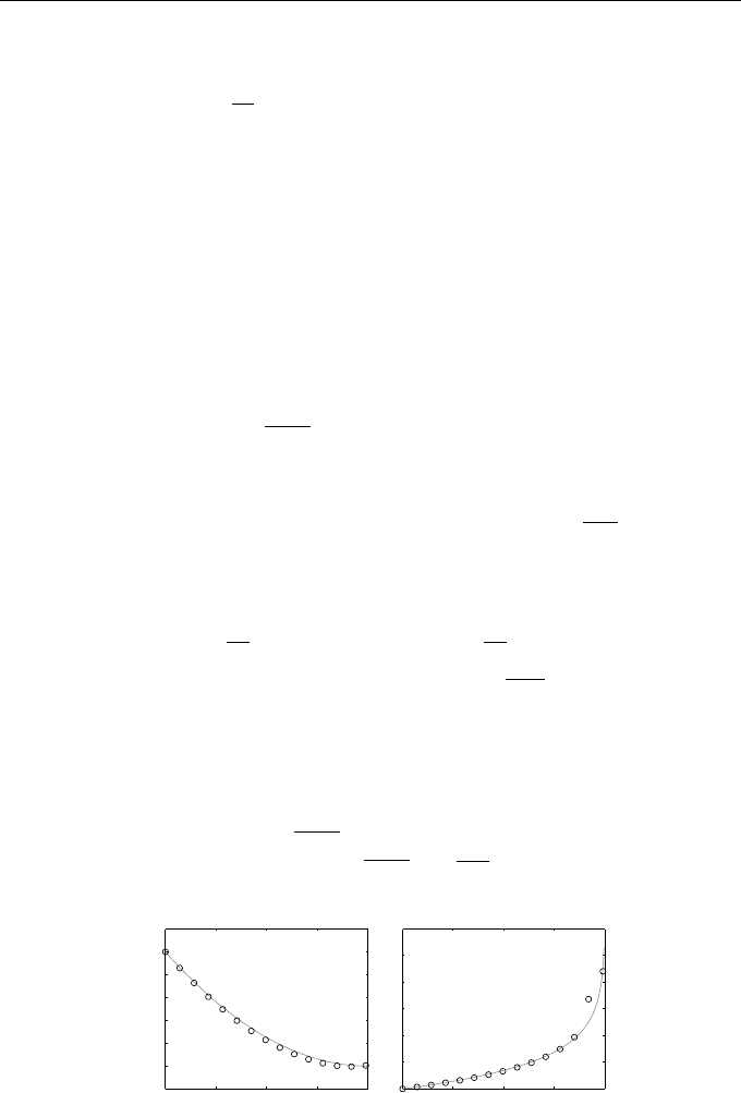
2/tol time steps. Sample numerical results are

presented in Figure 13.5 (

2/tol =

√

200 ≈ 14.14 and x

= 0.0046.

0 0.5 1 1.5 2

−0.2

0.2

0.4

0.6

0.8

1.2

0 0.5 1 1.5 2

Fig. 13.5 Numerical solution for Exercise 13.12 with λ = 1 and tol = 0.01.

Left: (s

, x

) (Circles) and (s, x(s)) (solid), Right: (s

, t

) (circles) and (s, t(s))

(solid)

Geometric Integration Part I—Invariants

14.1 Introduction

We judge a numerical method by its ability to “approximate” the ODE. It is

perfectly natural to

– ﬁx an initial condition,

– ﬁx a time t

and ask how closely the method can match x(t

), perhaps in the limit h → 0.

This led us, in earlier chapters, to the concepts of global error and order of

convergence. However, there are other senses in which approximation quality

may be studied. We have seen that absolute stability deals with long-time be-

haviour on linear ODEs, and we have also looked at simple long-time dynamics

on nonlinear problems with ﬁxed points. In this chapter and the next we look

at another well-deﬁned sense in which the ability of a numerical method to re-

produce the behaviour of an ODE can be quantiﬁed—we consider ODEs with a

conservative nature—that is, certain algebraic quantities remain constant (are

conserved) along trajectories. This gives us a taste of a very active research area

that has become known as geometric integration, a term that, to the best of our

knowledge, was coined by Sanz-Serna in his review article [60]. The material in

these two chapters borrows heavily from Hairer et al. [26] and Sanz-Serna and

Calvo [61].

Throughout both chapters, we focus on autonomous ODEs, where the right-

hand side does not depend explicitly upon t, so we have x

(t) = f (x).

Springer Undergraduate Mathematics Series, DOI 10.1007/978-0-85729-148-6_14,

D.F. Griffiths, D.J. Higham, Numerical Methods for Ordinary Differential Equations,