Griffiths D.F., Higham D.J. Numerical Methods for Ordinary Differential Equations: Initial Value Problems

Подождите немного. Документ загружается.

206 14. Geometric Integration Part I—Invariants

14.11.

By directly diﬀerentiating, show that H in (14.17) is an invariant

for the Kepler problem (14.15).

14.12.

???

(Based on Gonzalez et al. [22, Section 4.6].) Consider the scalar

ODE x

(t) = f (x(t)), with f(x) = −x

. Letting F(x) = x

/4, use

the chain rule to show that

F(x(t)) = −(f (x(t)))

. (14.26)

Deduce that

lim

t→∞

x(t) = 0, for any x(0).

For this ODE, rather than being an invariant, F is a Lyapunov func-

tion that always decreases along each non-constant trajectory. For

the backward Euler method x

n+1

= x

−hx

n+1

, by using the Taylor

series with remainder it is possible to prove a discrete analogue of

(14.26),

F(x

n+1

) − F(x

)

≤ −



n+1

− x



It follows that, given any h,

lim

n→∞

= 0, for any x(0).

Show that

(t) = −y

(t) +

(t)

is a modiﬁed equation for backward Euler on this ODE, and also

deduce that

lim

t→∞

|y(t)| = ∞, when y(0) >

This gives an example of a qualitative property that is shared by an

ODE and a numerical method for all h, but is not inherited by a

corresponding modiﬁed equation.

Geometric Integration Part

II—Hamiltonian Dynamics

This chapter continues our study of geometric features of ODEs. We look at

Hamiltonian problems, which possess the important property of symplecticness.

As in the previous chapter our emphasis is on

– showing that methods must be carefully chosen if they are to possess the

correct geometric property, and

– using the idea of modiﬁed equations to explain the qualitative behaviour of

numerical methods.

15.1 Symplectic Maps

As a lead-in to the topics of Hamiltonian ODEs and symplectic maps, we be gin

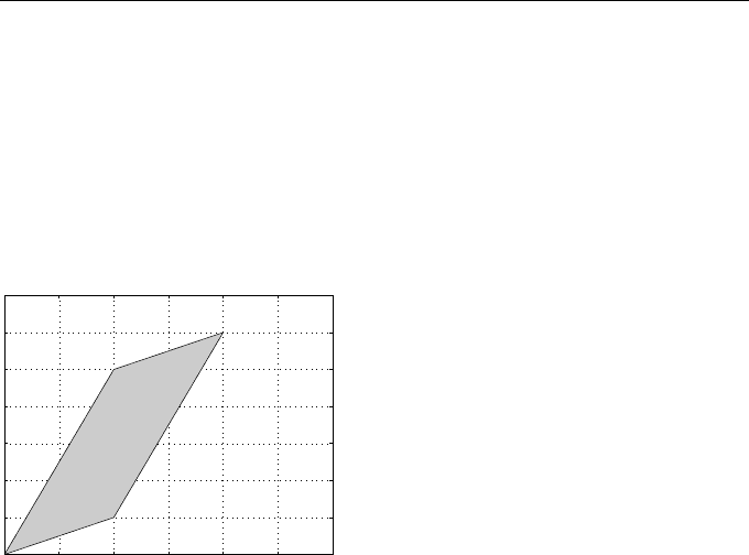
with some key geometric concepts. Figure 15.1 depicts a parallelogram with

vertices at (0, 0), (a, b), (a + c, b + d), and (c, d). The area of the parallelogram

can be written as |ad − bc|; see Exercise 15.1. If we remove the absolute value

sign, then the remaining expression ad − bc is positive if the vertices are listed

in clockwise order, otherwise it is negative. Hence, characterizing the parallel-

ogram in terms of the two vectors

u =





and v =





Springer Undergraduate Mathematics Series, DOI 10.1007/978-0-85729-148-6_15,

D.F. Griffiths, D.J. Higham, Numerical Methods for Ordinary Differential Equations,

208 15. Geometric Integration Part II—Hamiltonian Dynamics

we may deﬁne the oriented area, area

(u, v), to be ad − bc. Equivalently, we

may write

area

(u, v) = u

Jv, (15.1)

where J ∈ R

2×2

has the form

J =



0 1

−1 0



(a,b)

(a+c,b+d)

(c,d)

Fig. 15.1 Parallelogram

Now, given a matrix A ∈ R

2×2

, we may ask whether the oriented-area is

preserved under the linear mapping u 7→ Au and v 7→ Av. From (15.1), we will

have area

(u, v) = area

(Au, Av) if and only if u

JAv = u

Av. Hence,

the linear mapping guarantees to preserve oriented area if, and only if,

JA = J. (15.2)

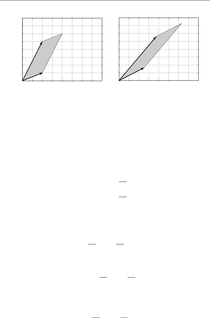
Figure 15.2 illustrates this idea. Here, the parallelogram on the right is found

by applying a linear mapping to u and v, and, since we have chosen a matrix

A for which A

JA = J, the oriented area is preserved. We also note that the

condition (15.2) is equivalent to det(A) = 1; see Exercise 15.5. However, we

prefer to use the formulation (15.2) as it is convenient algebraically and, for

our purposes, it extends more naturally to the case of higher dimensions.

Adopting a more general viewpoint, we may consider any smooth nonlinear

mapping g : R

→ R

. When is g oriented area preserving? In other words,

if we take a two-dimensional region and apply the map g to every point, this

will give us a new region in R

. Under what conditions will the two regions

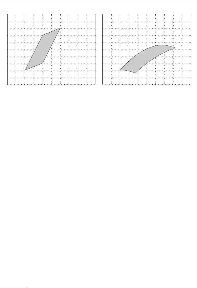
always have the same oriented area? Fixing on a point x ∈ R

, we imagine a

small parallelogram formed by the vectors x + ε and x + δ, where ε, δ ∈ R

are arbitrary but small, as indicated in the left-hand picture of Figure 15.3.

Placing the origin at x, we know from (15.1) that the oriented area of this

parallelogram is given by

Jδ. (15.3)

15.1 Symplectic Maps 209

u + v

Au + Av

Fig. 15.2 The parallelogram on the right was formed by using a matrix A to

map the vectors u and v that deﬁne the edges of the parallelogram on the le ft.

In this case det(A) = 1, so the area is preserved

If we apply the map g to this parallelogram then we get a region in R

, as

indicated in the right-hand picture. Because ε and δ are small, the sides of

this region can be approximated by straight lines, and the new region can be

approximated by a parallelogram. Also, by linearizing the map, as explained

in Appendix C, we may approximate the locations of the vertices g(x + ε) and

g(x + δ) using (C.3) to obtain

g(x + ε) ≈ g(x) +

∂g

∂x

(x) ε,

g(x + δ) ≈ g(x) +

∂g

∂x

(x) δ.

Here the Jacobian ∂g/∂x is the matrix of partial derivatives, see (C.4). Placing

the origin at g(x), the oriented area of this region may be approximated by

the oriented area of the parallelogram, to give



∂g

∂x





∂g

∂x



δ. (15.4)

Equating the oriented areas (15.3) and (15.4) gives the relation

Jδ = ε



∂g

∂x





∂g

∂x



δ.

Now the directions ε and δ are arbitrary, and we would like this area preser-

vation to hold for any choices. This leads us to the condition

J =



∂g

∂x





∂g

∂x



. (15.5)

The ﬁnal step is to argue that any region in R

can be approximated to any

desired level of accuracy by a collection of small parallelograms. Hence, this

210 15. Geometric Integration Part II—Hamiltonian Dynamics

x + ǫ

x + δ

g(x)

g(x + ε)

g(x + δ)

Fig. 15.3 The region on the right illustrates the eﬀect of applying a smooth

nonlinear map g to the set of points making up the parallelogram on the left.

If the original parallelogram is small, then the map is well approximated by its

linearisation (equivalently, the new region is well approximated by a parallelo-

gram).

condition is enough to guarantee area preservation in general. These arguments

can be made rigorous and a smooth map g satisfying condition (15.5) does

indeed preserve oriented area.

We will use the word symplectic to denote maps that satisfy (15.5).

15.2 Hamiltonian ODEs

With a unit mass and unit gravitational constant the motion of a pendulum

can be modelled by the ODE system

(t) = −sin q(t),

(t) = p(t).

(15.6)

Here, the position coord inate, q(t), denotes the angle between the rod and the

vertical at time t.

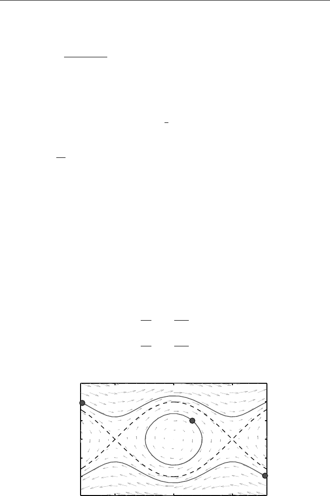
Figure 15.4 shows solutions of this system in the q, p phase space. In each

case, the initial condition is marked with a circle. We have also indicated the

For maps in R

where d > 1, the concept of symplecticness is stronger than

simple preservation of volume—it is equivalent to preserving the sum of the oriented

areas of projections on to two-dimensional subspaces. However, the characterization

(15.5) remains valid when the matrix J is generalized appropriately to higher di-

mension, and the algebraic manipulations that we will use can be carried through

automatically.

15.2 Hamiltonian ODEs 211

vector ﬁeld for this system—an arrow shows the direction and size of the tan-

gent vector for a solution passing through that point. In other words, an arrow

at the point (q, p) has direction given by the vector (p, −sin q) and length pro-

portional to

+ sin

q. There is a ﬁxed point at p = q = 0, corresponding

to the pendulum resting in its lowest position, and an unstable ﬁxed point at

q = π, p = 0, c orresponding to the pendulum resting precariously in its highest

position. For any solution, the function

H(p, q) =

− cos q (15.7)

satisﬁes

H(p, q) = pp

+ (sin q)q

= −p sin q + (sin q)p = 0.

Hence, H(p, q) remains constant along each solution. In fact, for −1 < H < 1,

we have the typical “grandfather clock” libration—solutions where the angle

q oscillates between two ﬁxed values ±c. One such solution is shown towards

the centre of Figure 15.4. For H > 1, the angle q varies monotonically; here,

the pendulum continually swings beyond the vertical. Two of these solutions

are shown in the upper and lower regions of the ﬁgure. The intermediate case,

H = 1, corresponds to the unstable resting points and the separatrices that

connect them are marked with dashed lines (see Exercise 15.8). We also note

that the problem is 2π periodic in the angle q.

The pendulum system (15.6) may be written in terms of the function H :

→ R

in (15.7) as

= −

∂H

∂q

∂H

∂p

(15.8)

−3

−2

−1

−π

Fig. 15.4 Vector ﬁeld and particular solutions of the pendulum system (15.6).

212 15. Geometric Integration Part II—Hamiltonian Dynamics

It turns out that many other important ODE systems can also be written in

this special form (or higher-dimensional analogues, as in the Kepler example

(14.18)). Hence, this class of problems is worthy of special attention. Generally,

any system of the form (15.8) is called a Hamiltonian ODE and H(p, q) is

referred to as the corresponding Hamiltonian function. The invariance of H

that we saw for the pendulum example carries through, be cause , by the chain

rule,

H(p, q) =

∂H

∂p

∂H

∂q

= −

∂H

∂p

∂H

∂q

∂H

∂q

∂H

∂p

= 0.

However, in addition to preserving the Hamiltonian function, these problems

also have a symplectic character. To see this, we need to introduce the time t

ﬂow map, ψ

, which takes the initial condition p(0) = p

, q(0) = q

and maps

it to the solution p(t), q(t); that is,







p(t)

q(t)



Once we have ﬁxed t, this deﬁnes a map ψ

: R

→ R

, and we may therefore

investigate whether this map preserves oriented area.

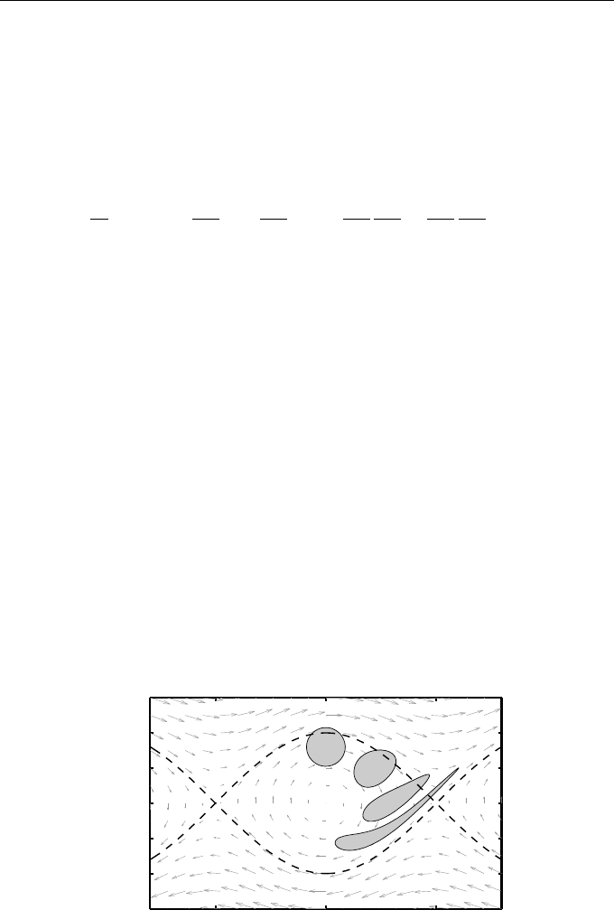
Before carrying this out, the results of a numerical experiment are displayed

in Figure 15.5. The eﬀ ec t of applying ψ

to all the points in the shaded circular

disc with centre at q = 0, p = 1.6 and radius 0.55 is shown for t = 1 and t = 2

and t = 3. In other words, taking every point in the disk as an initial value for

the ODE system, we show where the solution lies at times t = 1, 2, 3. At time

t = 1, the disk is rotated clockwise and squashed into a distorted egg shape.

At time t = 2 the region is stretched into a teardrop by the vector ﬁeld, and

by t = 3 it has taken on a tadpole shape.

−3

−2

−1

−π

Fig. 15.5 Illustration of the area-preserving property for the ﬂow of the pen-

dulum system (15.6)

15.2 Hamiltonian ODEs 213

It would be reasonable to conjecture from Figure 15.5 that the time t ﬂow

map ψ

is symplectic—the shaded regions app e ar to have equal areas. To pro-

vide a proof we use the approach used in the previous section with g(x) ≡ ψ

(x)

and x = [p, q]

. We ﬁrst note that, for t = 0, ψ

collapses to the identity map,

so its Jacobian (C.4) is the identity matrix, which trivially satisﬁes (15.5). Next,

we consider how the right-hand side of (15.5) evolves over time. The Jacobian

matrix (C.7) for (15.6) has the form



0 −cos q

1 0



Then, letting

P (t) =

∂ψ

∂x

denote the matrix of partial derivatives, the variational equation for this matrix

has the form

(t) =



0 −cos q

1 0



P (t)

(see (C.6)). It follows that



P (t)

JP (t)



= P

(t)

JP (t) + P (t)

(t)

= P (t)



0 1

−cos q 0



0 1

−1 0



P (t)

+ P (t)



0 1

−1 0



0 −cos q

1 0



P (t)

= P (t)



−1 0

0 −cos q





1 0

0 cos q



P (t)

= 0. (15.9)

Having ﬁrst e stablished that (15.5) holds at time t = 0, we have now shown that

the right-hand side of (15.5) does not change over time; hence, the condition

holds for any time t. That is, the time t ﬂow map, ψ

, for the pendulum equation

is symplectic for any t.

The general case, where H(p, q) is any Hamiltonian function in (15.8), can

be handled without much more eﬀort. The ODE then has a Jacobian of the

form



−H



Here, we have adopted the compact notation where, for example, H

denotes

∂

H /∂p∂q. This Jacobian may be written as J

−1

∇

H, where

−1



0 −1

1 0



and ∇

H =





214 15. Geometric Integration Part II—Hamiltonian Dynamics

Here, the symmetric m atrix ∇

H is called the Hessian of H. The computations

leading up to (15.9) then generalise to



P (t)

JP (t)



= P

(t)

JP (t) + P (t)

(t)

= P (t)

∇

−T

JP (t) + P (t)

∇

HP (t) = 0,

since J

−T

J = −I. So the argument used for the pendulum ODE extends to

show that any Hamiltonian ODE has a symplectic time t ﬂow map, ψ

15.3 Approximating Hamiltonian ODEs

We will describe two examples of approximating systems of Hamiltonian ODEs.

Example 15.1

Show that map generated when Euler’s method is applied the pendulum ODEs

(15.6) is not symplectic.

Euler’s method corresponds to the map



n+1





− h sin q

+ hp



. (15.10)

We ﬁnd that







∂p

n+1

∂p

n+1

∂q

n+1

∂p

∂q

n+1

∂q









1 −h cos q

h 1



and the right-hand side of (15.5) is



0 1 + h

cos q

−1 − h

cos q



Since this is not the identity matrix, the map arising from Euler’s method on

this ODE is not symplectic for any step size h > 0.

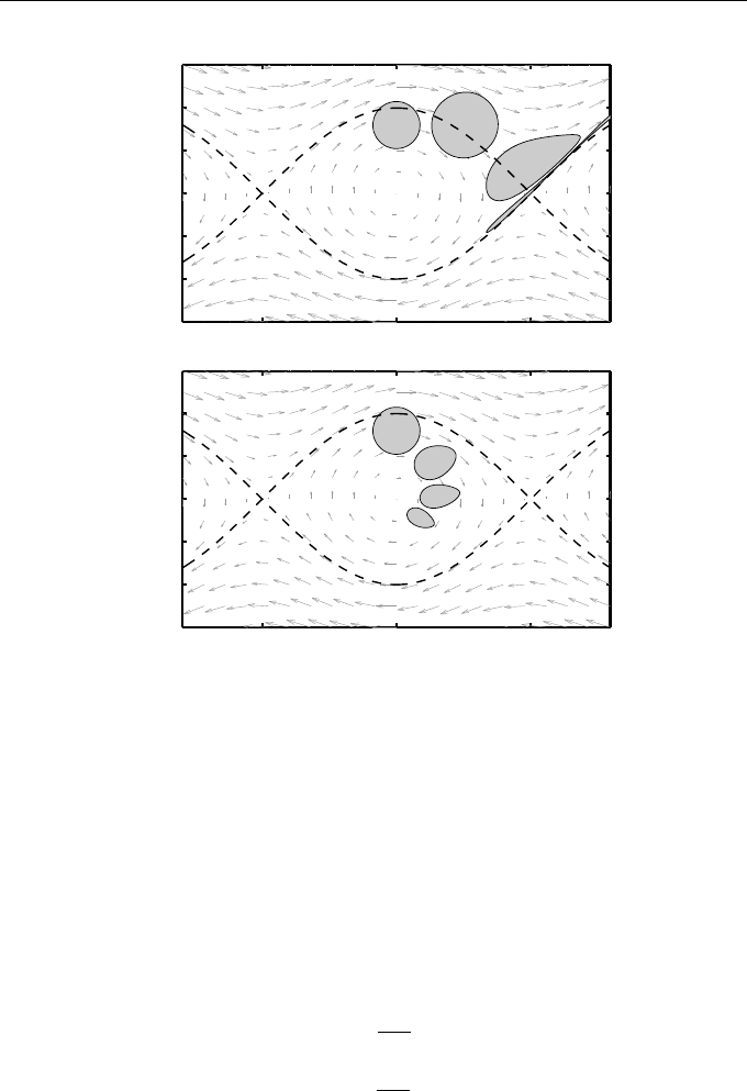
Figure 15.6 (top) shows what happens when the exact ﬂow map in Fig-

ure 15.5 is replaced by the Euler m ap (15.10) with step size h = 1. The disk

of initial values clearly starts to expand its area, before collapsing into a thin

smear. Figure 15.6 (bottom) repeats the experiment, this time using the back-

ward Euler method. Here, the region spirals towards the origin, and the area

appears to shrink. Exercise 15.7 asks you to check that the corresponding map

is not symplectic.

15.3 Approximating Hamiltonian ODEs 215

−3

−2

−1

−π

−3

−2

−1

−π

Fig. 15.6 Area evolution for the forward Euler method (top) and backward

Euler method (bottom) applied to the pendulum system (15.6)

Example 15.2

Extend the s ymplectic Euler me thod from Example 13.4 to the general Hamil-

tonian system of ODEs (15.8) and verify that the resulting map is symplectic.

The symplectic Euler method can be regarded as a combination of forward

and backward Euler methods where the updates are implicit in the p variable

and explicit in the q variable. When applied to the system (15.8) it leads to

n+1

= p

− h

∂H

∂q

n+1

, q

n+1

= q

+ h

∂H

∂p

n+1

, q

(15.11)