Griffiths D.F., Higham D.J. Numerical Methods for Ordinary Differential Equations: Initial Value Problems

Подождите немного. Документ загружается.

226 16. Stochastic Diﬀerential Equations

an active research topic. Our aim here is to give a nontechnical and accessible

introduction, in the manner of the expository article by Higham [31]. For further

information, in roughly increasing order of technical diﬃculty, we recommend

Mikosch [51], Cyganowski et al. [13], Mao [49], Milsein and Tretyakov [52] and

Kloeden and Platen [42].

16.2 Random Variables

In this chapter, we deal informally with scalar continuous ra ndom variables,

which take values in the range (−∞, ∞). We may characterize such a random

variable, X, by the probability that X lies in any interval [a, b]:

P (a ≤ X ≤ b) =

p(y) dy. (16.1)

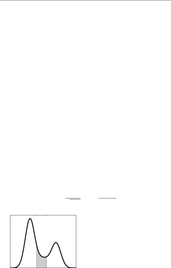
Here, p is known as the probability density function for X, and the left-hand side

of (16.1) is read as “the probability that X lies between a and b.” Figure 16.1

illustrates this idea: the chance of X taking values between a and b is given

by the corresponding area under the curve. So regions where the density p is

large correspond to likely values. Because probabilities cannot be negative, and

because X must lie somewhere, a density function p must satisfy

(a) p(y) ≥ 0, for all y ∈ R;

(b)

∞

−∞

p(y) dy = 1.

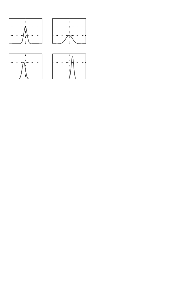
An extremely important case is

p(y) =

√

2σ

exp



−

(y − µ)

2σ



, (16.2)

a b

p(y)

Fig. 16.1 Illustration of the identity

(16.1). The probability that X lies be-

tween a and b is given by the area un-

der the probability density function for

a ≤ y ≤ b

16.2 Random Variables 227

−10 0 10

0.2

0.4

µ = 0, σ = 1

p (y )

−10 0 10

0.2

0.4

µ = 0, σ = 2

p (y )

−10 0 10

0.2

0.4

µ = −1, σ = 1

p (y )

−10 0 10

0.2

0.4

µ = 2, σ = 0. 75

p (y )

Fig. 16.2 Some density functions

(16.2) corresponding to normally dis-

tributed random variables

where µ and σ ≥ 0 are ﬁxed parameters. Examples with µ = 0 and σ = 1,

µ = 0 and σ = 2, µ = −1 and σ = 1, and µ = 2 and σ = 0.75 are plotted

in Figure 16.2. If X has a probability density function given by (16.2) then we

write X ∼ N(µ, σ

) and say that X is a normally distributed random variable.

In particular, when X ∼ N(0, 1) we say that X has the standard normal distri-

bution. The bell-shaped nature of p in (16.2) turns out to be ubiquitous—the

celebrated Central Limit Theorem says that, loosely, whenever a large number

of random sources are combined whatever their individual nature, the overall

eﬀect can be well approximated by a single normally distributed random vari-

able.

The parameters µ and σ in (16.2) play well-deﬁned roles. The value y =

µ corresponds to a peak and an axis of symmetry of p, and σ controls the

“spread.” More generally, given a random variable X with probability density

function p, we deﬁne the mean, or expected value, to be

E[X] :=

∞

−∞

y p(y) dy. (16.3)

It is easy to check that E[X] = µ with the normal density (16.2); see Exer-

cise 16.1. The variance of X may then be deﬁned as the expected value of the

new random variable (X − E[X])

; that is,

var[X] := E

(X − E[X])

. (16.4)

Intuitively, the size of the variance captures the extent to which X may vary

about its mean. In the normal case (16.2) we have var[X] = σ

; see Exer-

cise 16.3.

The word normal here does not imply “common” or “typical”; it stems from the

geometric concept of orthogonality.

In this informal treatment, any integral that we write is implicitly assumed to

take a ﬁnite value.

228 16. Stochastic Diﬀerential Equations

16.3 Computing with Random Variables

A pseudo-random number generator is a computational algorithm that gives us

a new number, or sample, each time we reques t one. En masse, these samples

appear to agree with a speciﬁed density function. In other words, recalling

the picture in Figure 16.1, if we call the pseudo-random numbe r generator

lots of times, then the proportion of samples in any interval [a, b] would be

approximately the same as the integral in (16.1). If we think of each sample

coming out of the pseudo-random number generator as be ing the result of

an independent trial, then we can make the intuitively reasonable connection

between the probability of the event a ≤ X ≤ b and the frequency at which

that event is observed over a long sequence of independent trials. For example,

if a and b are chosen such that P (a ≤ X ≤ b) =

, then, in the long term, we

would expect half of the calls to a suitable pseudo-random number generator

to produce samples lying in the interval [a, b].

In this b ook we will assume that a pseudo-random number generator corre-

sponding to a random variable X ∼ N(0, 1) is available. For example, Matlab

has a built-in function randn, and 10 calls to this function produced the samples

-0.4326

-1.6656

0.1253

0.2877

-1.1465

1.1909

1.1892

-0.0376

0.3273

0.1746

and another ten produced

-0.1867

0.7258

-0.5883

2.1832

-0.1364

0.1139

1.0668

0.0593

-0.0956

-0.8323

16.3 Computing with Random Variables 229

Supp ose we generate M samples from randn. We may divide the y-axis into

bins of length ∆

and let N

denote the number of samples in each subinterval

[i∆

, (i + 1)∆

]. Then the integral-based deﬁnition of probability (16.1) tells us

that

P (i∆

≤ X ≤ (i + 1)∆

) =

(i+1)∆

i∆

p(y) dy ≈ p(i∆

)∆

. (16.5)

This was obtained by approximating the area under the curve by the area of

a rectangle with height p(i∆

) and base ∆

; this is valid when ∆

is small.

On the other hand, identifying the probability of an event with its long-term

observed frequency, we have

P (i∆

≤ X ≤ (i + 1)∆

) ≈

. (16.6)

Combining (16.5) and (16.6) gives us

p(i∆

) ≈

∆

. (16.7)

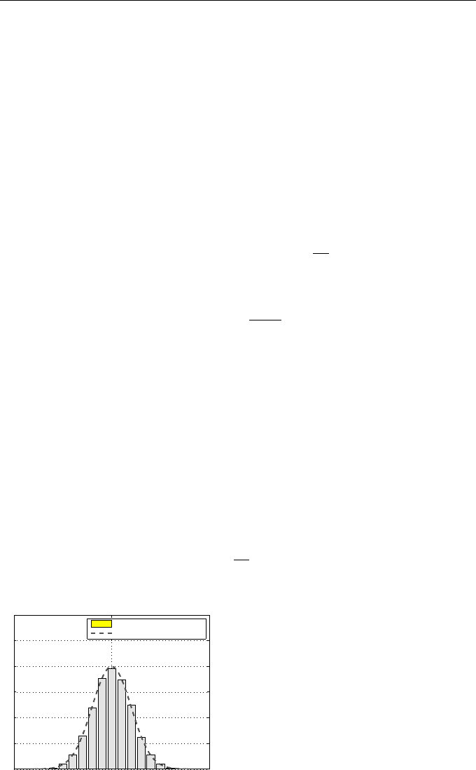
Figure 16.3 makes this concrete. Here, we took M = 10000 samples from Mat-

lab’s randn and used 17 subintervals on the y-axis, with centres at −4, −3.5,

−3, . . . , 3.5, 4. The histogram shows the appropriately scaled proportion of

samples lying in each interval; the height of each rectangle is given by the

right-hand side of (16.7). We have superimposed the probability density func-

tion (16.2) with µ = 0 and σ = 1, which is seen to match the computed data.

In many circumstances, our aim is to ﬁnd the exp ec ted value of some random

variable, X, and we are able to use a pseudo-random number generator to

compute samples from its distribution. If {ξ

}

i=1

is a set of such samples, then

it is intuitively reas onable that the sample mean

i=1

(16.8)

−5 0 5

0.1

0.2

0.3

0.4

0.5

pseudo -ran d om data

N(0,1) d ensity

Fig. 16.3 Histogram of s amples from

a N(0, 1) pseudo-random number gener-

ator, with probability density function

(16.2) for µ = 0 and σ = 1 superim-

posed. This illustrates the idea that e n

masse the samples appear to come from

the appropriate distribution

230 16. Stochastic Diﬀerential Equations

can be used to approximate E[X]. Standard statistical results

can be used to

show that in the asymptotic M → ∞ limit, the range

−

1.96

var[X]

√

, a

1.96

var[X]

√

(16.9)

is a 95% conﬁdence interval for E[X]. This may be understood as follows: if we

were to repeat the computation of a

in (16.8) many times, each time using

fresh samples from our pseudo-random number generator, then the statement

“the exact mean lies in this interval” would be true 95% of the time. In practice,

we typically do not have access to the exact variance, var[X], which is required

in (16.9). From (16.4) we see that the variance is itself a particular case of

an expected value, so the idea in (16.8) can be repe ated to give the sample

variance

i=1

(ξ

− a

)

Here, the unknown expected value E[X] has been replaced by the sample mean

Hence, instead of (16.9) we may use the more practical alternative

−

1.96

√

, a

1.96

√

. (16.10)

As an illustration, consider a random variable of the form

X = e

−1+2Y

, where Y ∼ N(0, 1).

In this case, we can com pute samples by calling a standard normal pseudo-

random number generator, scaling the output by 2 and shifting by −1 and

then exponentiating. Table 16.1 s hows the sample means (16.8) and conﬁdence

intervals (16.10) that arose when we used M = 10

, 10

, . . . , 10

. For this simple

example, it can be shown that the exact mean has the value E[X] = 1 (see

Exercise 16.4) so we can judge the accuracy of the results. Of course, this

type of computation, which is known as a Monte Carlo simulation, is useful in

those circumstances where the exact mean cannot be obtained analytically. We

see that the accuracy of the sample mean and the precision of the conﬁdence

interval improve as the number of samples, M , increases. In fact, we can see

directly from the deﬁnition (16.10) that the width of the conﬁdence interval

scales with M like 1/

√

M; so, to obtain one more decimal place of accuracy we

need to do 100 times more computation. For this reason, Monte Carlo simulation

is impractical when very high accuracy is required.

More precisely, the Strong L aw of Large Numbers and the Central Limit Theo-

rem.

There is a well-deﬁned sense in which this version of the sample variance is

improved if we multiply it by the factor M/(M −1). However, a justiﬁcation for this

is beyond the scope of the book, and the eﬀect is negligible when M is large.

16.4 Stochastic Diﬀerential Equations 231

M a

conﬁdence interval

0.9445 [0.4234, 1.4656]

0.8713 [0.6690, 1.0737]

1.0982 [0.9593, 1.2371]

1.0163 [0.9640, 1.0685]

0.9941 [0.9808, 1.0074]

1.0015 [0.9964, 1.0066]

Table 16.1 Sample means and conﬁdence intervals for Monte Carlo simula-

tionsof a random variable X for which E[X] = 1

16.4 Stochastic Diﬀerential E quations

We know that the Euler iteration

n+1

= x

+ hf (x

)

produces a sequence {x

} that converges to a solution of the ODE x

(t) =

f(x(t)). To introduce a stochastic e leme nt we will give each x

n+1

a random

“kick,” so that

n+1

= x

+ hf (x

) +

√

h ξ

g(x

). (16.11)

Here, ξ

denotes the result of a call to a standard normal pseudo-random

number generator and g is a given function. So the size of the random kick is

generally state-dependent—it depends upon the current approximation x

, via

the value g(x

). We also see a factor

√

h in the random term. Why is it not

h, or h

1/4

or h

? It turns out that

√

h is the correct scaling when we consider

the limit h → 0. A larger power of h would cause the noise to disappear and

a smaller power of h would cause the noise to swamp out the original ODE

completely.

Given functions f and g and an initial condition x(0), we can think of a

process x(t) that arises when we take the h → 0 limit in (16.11). In other words,

just as in the deterministic case, we can ﬁx t and consider the limit as h → 0

of x

where Nh = t. Of course, this construction for x(t) leads to a random

variable—each set of pseudo-random numbers {ξ

}

N−1

n=0

gives us a new sample

from the distribution of x(t).

Assuming that this h → 0 limit is valid, we will refer to x(t) as the solution

to a stochastic diﬀerential equation (SDE). There are thus three ingredients for

an SDE

– A function f, which plays the same role as the right-hand side of an ODE.

In the SDE context this is called the drift coeﬃcient.

232 16. Stochastic Diﬀerential Equations

– A function g, which aﬀects the size of the noise contribution. This is known

as the diﬀusion coeﬃcient.

– An initial condition, x(0). The initial condition might be deterministic, but

more generally it is allowed to be a random variable—in that case we simply

use a pseudo-random number generator to pick the starting value x

for

(16.11).

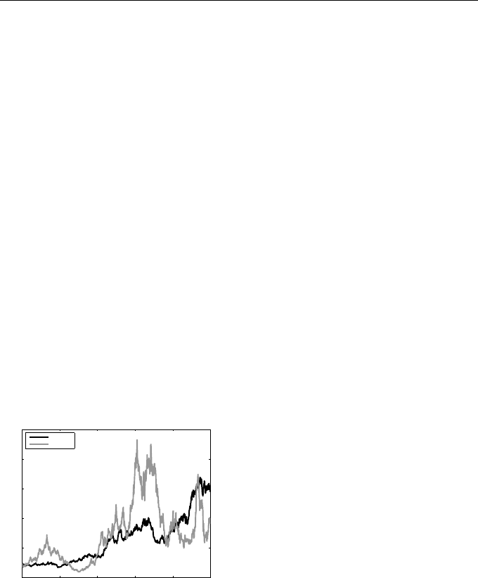
As an illustration, we will consider the case where f and g are linear; that

is,

f(x) = ax, g(x) = bx, (16.12)

where a and b > 0 are constants, and we ﬁx x(0) = 1. For the dark curve

in Figure 16.4 we take a = 2, b = 1, and x(0) = 1, and show the results of

applying the iteration (16.11) with a step size h = 10

−3

for 0 ≤ t ≤ 1. The

closely spaced, but discrete, points {x

} have been joined by straight lines for

clarity. This gives the impression of a continuous but jagged curve. This can

be formalized—the limiting h → 0 solution produces paths that are continuous

but nowhere diﬀerentiable. For the lighter curve in Figure 16.4 we repeated the

experiment with diﬀerent pseudo-random samples ξ

and with the diﬀusion

strength b increased to 2. We see that this gives a more noisy or “volatile”

path.

0 0.2 0.4 0.6 0.8 1

b = 1

b = 2

Fig. 16.4 Results for the iteration

(16.11) with drift and diﬀusion coef-

ﬁcients from (16.12) and a step size

h = 10

−3

. Here, for the same drift

strength, a = 2, we show a path with

b = 1 (dark) and b = 2 (light)

We emphasize that the details in Figure 16.4 would change if we repeated

the experiments with fresh pseudo-random numbers. To illustrate this idea, in

the upper picture of Figure 16.5 we show 50 diﬀerent paths, each computed

as in Figure 16.4, with a = 0.06 and b = 0.75. At the ﬁnal time, t = 1, each

path produces a single number that, in the h → 0 limit, may be regarded as a

sample from the distribution of the random variable x(1) describing the SDE

solution at t = 1. In the lower picture of Figure 16.5 we produced a histogram

for 10

such samples. Overall, the ﬁgure illustrates two diﬀerent ways to think

about an SDE. We can consider individual paths evolving over time, as in the

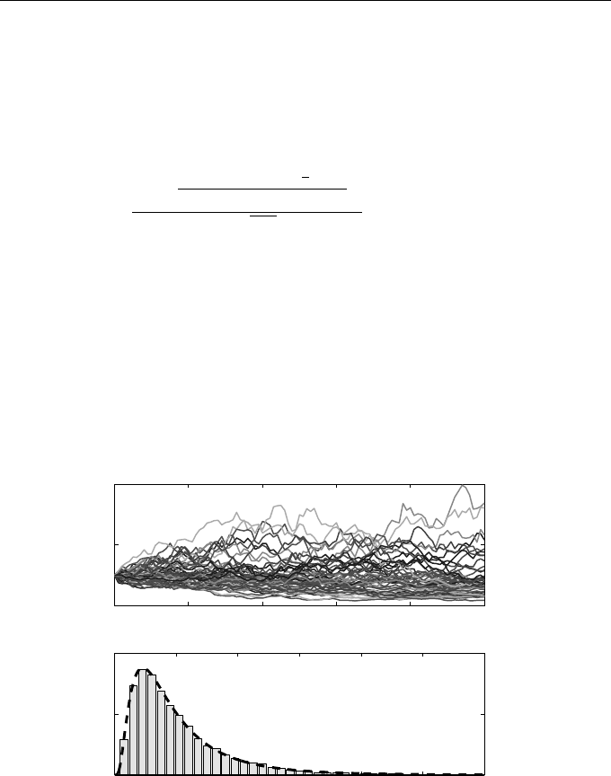
16.4 Stochastic Diﬀerential Equations 233

upp e r picture, or we can ﬁx a point in time and consider the distribution of

values at that point, as in the lower picture. From the latter p erspective, by

studying this simple SDE analytically it can be shown, given a deterministic

initial condition, that for the exact solution the random variable x(t) at time t

has a so-called lognormal probability density function given by

p(y) =

exp



−[log(y/x(0))−(a−

)t]



√

2πt

, for y > 0, (16.13)

and p(y) = 0 for y ≤ 0. We have superimposed this density function for t = 1

in the lower picture of Figure 16.5, and we see that it matches the histogram

closely. Exercise 16.6 asks you to check that (16.13) deﬁnes a valid density

function, and to conﬁrm that the mean and variance take the form

E[x(t)] = x

, (16.14)

var[x(t)] = x

2at



− 1



. (16.15)

0 0.2 0.4 0.6 0.8 1

50 paths

x( t)

0 1 2 3 4 5 6

0.5

samples from x(t) at t = 1

x( 1)

Fig. 16.5 Upper: In the manner of Figure 16.4, 50 paths using (16.11) for

the linear case (16.12) with a = 0.06 and b = 0.75. Lower: In the manner of

Figure 16.3, binned path values at the ﬁnal time t = 1 and probability density

function (16.13) superimposed as a dashed curve.

234 16. Stochastic Diﬀerential Equations

16.5 Examples of SDEs

In this section we mention a few examples of SDE models that have been

proposed in various application areas.

Example 16.1

In mathematical ﬁnance, SDEs are often used to represent quantities whose

future values are uncertain. The linear case (16.12) is by far the most popular

model for assets, such as company share prices, and it forms the basis of the

celebrated Black–Scholes theory of option valuation [32]. If b = 0 then we revert

to the simple deterministic ODE x

(t) = ax(t), for which x(t) = e

x(0). This

describes the growth of an inves tment that has a guaranteed ﬁxed rate a. The

stochastic term that arises when b 6= 0 reﬂects the uncertainty in the rate of

retur

n for a typical ﬁnancial asset.

In this context, b is called the volatility.

Example 16.2

A mean-reverting square-root process is an SDE with

f(x) = a (µ − x) , g(x) = b

√

x, (16.16)

where a, µ, and b > 0 are constants. For this SDE

E[x(t)] = µ + e

−at

(E[X(0)] − µ) (16.17)

(see Exercise 16.9) so we see that µ represents the long-term mean value. This

model is often used to represent an interest rate; and in this context it is as -

sociated with the names Cox, Ingersoll and Ross [11]. Given a positive initial

condition, it can be shown that the solution never becomes negative, so the

square root in the diﬀusion coeﬃcient, g(x), always makes sense. See, for ex-

ample, Kwok [43] and Mao [49] for more details.

Example 16.3

The traditional logistic ODE for population growth can be generalized to allow

for stochastic eﬀects by taking

f(x) = rx (K − x) , g(x) = βx, (16.18)

where r, K and β > 0 are constants. Here, x(t) denotes the population density

of a species at time t, with carrying capacity K and characteristic timescale

1/r [56], and β governs the strength of the environmental noise.

Or the authors’ pension funds.

16.5 Examples of SDEs 235

Example 16.4

The case where

f(x) = r (G − x) , g(x) =

εx (1 − x), (16.19)

with r, ε > 0 and 0 < G < 1 is suggested by Cobb [9] as a model for the motion

over time of an individual through the liberal–conservative political spectrum.

Here x(t) = 0 denotes an extreme liberal and x(t) = 1 denotes an extreme

conservative. With this choice of diﬀusion term, g(x), a person with extreme

views is less likely to undergo random ﬂuctuations than one nearer the centre

of the political spectrum.

Example 16.5

The SDE with

f(x) = −µ



1 − x



, g(x) = σ, (16.20)

with µ and σ > 0, is proposed by Lesmono et al. [46]. Here, in an environ-

ment where two political parties, A and B, are dominant, x(t) represents the

diﬀerence P

(t) −P

(t), where P

(t) and P

(t) denote the proportions of the

population that intend to vote for parties A and B, respectively, at time t.

Example 16.6

Letting V (x) denote the double-well potential

V (x) = x

(x − 2)

; (16.21)

as shown in Figure 16.6, we may construct the SDE with

f(x) = −V

(x), g(x) = σ. (16.22)

When σ = 0, we see from the chain rule that the resulting ODE x

(t) =

−V

(x(t)) satisﬁes

V (x(t)) = V

(x(t))

x(t) = −(V

(x(t)))

So, along any solution curve, x(t), the potential V (·) is nonincreasing. More-

over, it strictly decreases until it reaches a stationary point; with reference to

Figure 16.6, any solution with x(0) 6= 1 slides down a wall of the potential well

and

comes to rest at the appropriate minimum x = 0 or x = 2. In the additive

noise case, σ > 0, it is now possible for a solution to overcome the potential

barrier that se parates the two stable rest states—a path may occasionally jump