Griffiths D.F., Higham D.J. Numerical Methods for Ordinary Differential Equations: Initial Value Problems

Подождите немного. Документ загружается.

236 16. Stochastic Diﬀerential Equations

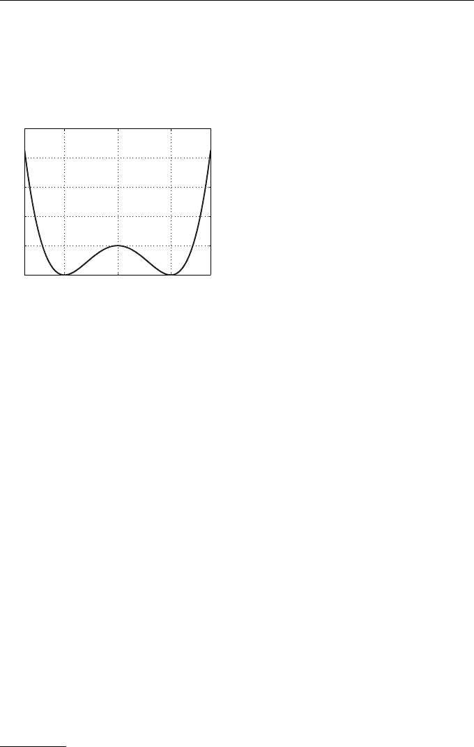
over the central hump and thereby move from the vicinity of one well to the

other. This gives a simple caricature of a bistable switching mechanism that is

important in biology and physics.

0 1 2

V (x)

Fig. 16.6 Double–well potential func-

tion V (x) from (16.21)

16.6 Convergence of a Numerical Method

Our informal approach here is to regard an SDE as whatever arises when we

take the h → 0 limit in the iteration (16.11). For any ﬁxed h > 0, we may then

interpret (16.11) as a numerical method that allows us to compute approxima-

tions for this SDE. In fact, this way of extending the basic Euler method gives

what is known as the Euler–Maruyama method. If we focus on the ﬁnal-time

value, t

, then we may ask how accurately the numerical method can approxi-

mate the random variable x(t

) from the SDE. For the example in Figure 16.5,

the lower picture shows that the histogram closely matches the correct density

function. Letting t

= nh, so that n → ∞ and h → 0 with t

ﬁxed, how can we

generalize the concept of order of convergence that we developed for ODEs?

It turns out that there are many, nonequivalent, ways in which to measure

the accuracy of the numerical method. If we let x

denote the random variable

corresponding to the numerical approximation at time t

, so that the endpoint

of each path in the upper picture of Figure 16.5 gives us a sample for x

then we could study the diﬀerence between the expected values of the random

variables x(t

) and x

. This quantiﬁes what is known as the weak error of the

method,

and it can be shown that this error decays at ﬁrst order; that is,

E [x(t

)] − E [x

] = O(h). (16.23)

More generally, the weak error can be deﬁned by comparing moments—expected

values of powers of x(t

) and x

16.6 Convergence of a Numerical Method 237

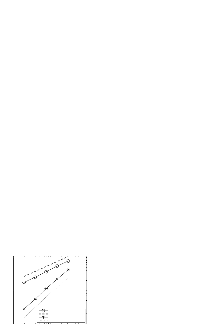
In Figure 16.7 we compute approximations to the weak error, as deﬁned in

the left-hand side of (16.23), for the linear SDE given by (16.12) with a = 2,

b = 1 and x(0) = 1. The asterisks show the weak error values for a range of

step sizes h. In each case, we used the known exact value (16.14) for the mean

of the SDE solution, and to approximate the mean of the numerical method we

computed a large number of paths and used the sample mean (16.8), making

sure that the 95% conﬁdence intervals were negligible relative to the actual

weak errors. Figure 16.7 uses a log-log scale, and the asterisks appear to lie

roughly on a straight line. A reference line with slope equal to one is s hown.

In the least-squares sense, the best straight line approximation to the asterisk

data gives a slope of 0.9858 with a residual of 0.0508. So, overall, the weak

errors are consistent with the ﬁrst-order behaviour quoted in (16.23).

The ﬁrst-order rate of weak convergence in (16.23) matches what we know

about the deterministic case—when we switch oﬀ the noise, g ≡ 0, the method

reverts to standard Euler, for which convergence of order 1 is attained.

On the other hand, if we are not concerned with “the error of the means”

but rather “the mean of the error,” then it may be more appropriate to look at

the strong error E[|x(t

) − x

|]. It can be shown that this version of the error

decays at a rate of only one half; that is,

E [|x(t

) − x

|] = O(h

1/2

). (16.24)

To make this concrete, for the same SDE and step sizes as in the weak tests,

the circles in Figure 16.7 show approximations to the strong error. Samples for

the “exact” SDE solution, x

, were obtained by following more highly resolved

paths—see, for example, Higham [31] for more information. The circles in the

ﬁgure appear to lie approximately on a straight line that agrees with the ref-

erence line of slope one half, and a least-squares ﬁt to the c ircle data gives a

slope of 0.5384 with residual 0.0266, consistent with (16.24).

We emphasize that this result marks a signiﬁcant departure from the deter-

ministic ODE case, where the underlying Euler method attains ﬁrst order. The

−3

−2

−1

−2

−1

Stron g o r Weak Error

St rong E rr or

Re f e renc e of slope 1/2

We ak E rror

Re f e renc e of slope 1

Fig. 16.7 Asterisks show weak er-

rors (16.23) and circles show strong er-

rors (16.24) for the Euler–Maruyama

method (16.11) applied to the linear

SDE (16.12)

238 16. Stochastic Diﬀerential Equations

degradation in approximation p ower when we measure error in the strong sense

of (16.24) is caused by a lack of smoothness that is evident from Figures 16.4

and 16.5; we cannot appeal directly to the type of Taylor series expansion

that s erved us so well in the preceding chapters, and a complete understanding

requires the tools of stochastic calculus.

16.7 Discussion

Although we have focussed here on scalar problems, the concept of SDEs ex-

tends naturally to the case of systems, x(t) ∈ R

, with multiple noise terms,

and the Euler–Maruyama method (16.11) carries through straightforwardly,

retaining the same weak and strong order.

For deterministic ODEs, Euler’s metho d would typically be dismissed as

having an order of convergence that is too low to be of practical use. For SDEs,

however, Euler–Maruyama, and certain low order implicit variations, are widely

used in practice. There are two good reasons.

1. Designing higher order methods is much more tricky, especially in the case

of systems, and those that have be en put forward tend to have severe

computational overheads.

2. Souping-up the iteration (16.11) is of limited use if the simulations are part of

a Monte Carlo style computation. In that case the relative ly slow O(1/

√

rate at which the conﬁdence interval shrinks is likely to provide the bottle-

neck.

Following up on point 2, we mention that recent work of Giles [21] makes it

clear that, in a Monte Carlo context, where we wish to compute the expected

value of a quantity involving the solution of an SDE,

– the concepts of weak and strong convergence are both useful, and

– it is worthwhile to study the interaction betwe en the weak and strong dis-

cretization errors arising from the timestepping method and the statistical

sampling error arising from the Monte Carlo method, in order to optimize

the overall eﬃciency.

Researchers in numerical methods for SDEs are actively pursuing many of

the issues that we have discussed in the ODE context, such as analysis of stabil-

ity, preservation of geometric features, construction of modiﬁed equations and

design of adaptive step size algorithms. There are also many new challenges, in-

cluding the development of multiscale methods that mix together deterministic

and stochastic regimes in order to model complex systems.

Exercises 239

EXERCISES

16.1.

Using the deﬁnition of the mean (16.3), show that E[X] = µ for

X ∼ N(µ, σ

). [Hint: you may use without proof the fact that

∞

−∞

p(y) dy = 1 for p(y) in (16.2).]

16.2.

Given that the expectation operator is linear, so that for any two

random variables X and Y and any α, β ∈ R,

E[αX + βY ] = αE[X] + βE[Y ], (16.25)

show that the variance, deﬁned in (16.4), may also be written

var[X] := E





− (E[X])

. (16.26)

16.3.

If the random variable X has probability density function p(y)

then, generally, for any function h, we have

E[h(X)] :=

∞

−∞

h(y) p(y) dy. (16.27)

Following on from Exercises 16.1 and 16.2 show that for X ∼

N(µ, σ

) we have E[X

] = µ

+ σ

and hence var[X] = σ

16.4.

Using h(y) = exp(−1 + 2y) in (16.27), show that E[X] = 1 for

X = exp(−1 + 2Y ) with Y ∼ N(0, 1).

16.5.

Based on the deﬁnition of the conﬁdence interval (16.10), if we did

not already know the exact answer, roughly how many more rows

would be needed in Table 16.1 in order for us to be 95% conﬁdent

that we have correctly computed the ﬁrst ﬁve signiﬁcant digits in

the expected value?

16.6.

Show that p(y) in (16.13) satisﬁes

∞

−∞

p(y) dy = 1 and, by eval-

uating

∞

−∞

y p(y) dy and

∞

−∞

p(y) dy, conﬁrm the expressions

(16.14) and (16.15).

16.7.

???

For the case where f(x) = ax and g(x) = bx, the Euler–Maruyama

method (16.11) takes the form

k+1

= (1 + ha) x

√

hbZ

, (16.28)

where each Z

∼ N(0, 1). Suppose the initial condition x(0) = x

is deterministic. By construction, we have E[Z

] = 0 and E[Z

] =

240 16. Stochastic Diﬀerential Equations

var[Z

] = 1. Because a fresh call to a pseudo-random number genera-

tor is made on each step, we can say that Z

and x

are independent,

and it follows that

E[x

] = E[x

]E[Z

] = 0,

E[x

] = E[x

]E[Z

] = 0,

E[x

] = E[x

]E[Z

] = E[x

Taking e xpectations in (16.28), and using the linearity property

(16.25), we ﬁnd that

E [x

k+1

] = E

(1 + ha) +

√

hbx

= (1 + ha) E[x

] +

√

hbE[x

]

= (1 + ha) E[x

So,

E [x

] = (1 + ha)

Consider now the limit where h → 0 and n → ∞ with nh = t

ﬁxed,

as in the convergence analysis of Theorem 2.4. Show that

E [x

] → e

, (16.29)

in agreement with the expression (16.14) for the SDE.

Similarly, squaring both sides in (16.28) and then taking expected

values, and using the linearity property (16.25), we have



k+1



= E

(1 + ha)

+ 2 (1 + ha)

√

hbx

+ hb

= (1 + ha)





+ 2 (1 + ha)

√

hbE





+ hb





= (1 + ha)





+ 0 + hb







(1 + ha)

+ hb







By taking logarithms, or otherwise, show that in the same limit

h → 0 and n → ∞ with nh = t

ﬁxed we have





→ e

(2a+b

so that

var[x

] = e

2at



− 1



in agreement with the expression (16.15) for the SDE.

Exercises 241

16.8.

???

Repeat the steps in Exercise 16.7 to get expressions for the mean

and variance in the additive noise case where f (x) = ax and g(x) =

b. This is an example of an Ornstein–Uhlenbeck process.

16.9.

Follow the arguments that led to (16.29) in order to justify the

expression (16.17) for the mean-reverting square root process.

Glossary and Notation

AB: Adams–Bashforth—names of a family of explicit LMMs. AB(2) denotes

the two-step, second-order Adams–Bashforth method.

AM: Adams–Moulton—names of a family of implicit LMMs. AM(2) denotes

the two-step, third-order Adams–Moulton method.

BDF: backward diﬀerentiation formula.

BE: backward Euler (method).

p+1

: error constant of a pth-order LMM.

CF: complementary function—the general solution of a homogeneous linear

diﬀerence or diﬀerential equation.

4E: diﬀerence equation.

E(·) : expected value.

: the value of f (t, x) at t = t

and x = x

FE: forward Euler (method).

GE: global error—the diﬀerence between the exact solution x(t

) at t = t

and the numerical solution x

: e

= x(t

) − x

∇: gradient operator. ∇F denotes the vector of partial derivatives of F.

h: step size—numerical solutions are sought at times t

= t

+ nh for n =

0, 1, 2, . . . .

Springer Undergraduate Mathematics Series, DOI 10.1007/978-0-85729-148-6,

D.F. Griffiths, D.J. Higham, Numerical Methods for Ordinary Differential Equations,

244 A. Glossary and Notation

h : λh, where λ is the coeﬃcient in the ﬁrst-order equation x

(t) = λx(t) or an

eigenvalue of the matrix A in the system of ODEs x

(t) = Ax(t).

I: identity matrix.

=(λ): imaginary part of a complex number λ.

IAS: interval of absolute stability.

IC: initial condition.

IVP: initial value problem—an ODE together with initial condition(s).

j = m : n: for integers m < n this is shorthand for the sequence of consecutive

integers from m to n. That is, j = m, m + 1, m + 2, . . . , n.

: linear diﬀerence operator.

LMM: linear multistep method.

LTE: local truncation error—generally the remainder term R in a Taylor series

expansion.

ODE: ordinary diﬀerential equation.

P(a ≤ X ≤ b): probability that X lies in the interval [a, b].

PS: particular solution—any solution of an inhomogeneous linear diﬀerence or

diﬀerential equation.

ρ(r): ﬁrst characteristic polynomial of a LMM.

R: region of absolute stability.

: interval of absolute stability.

<(λ): real part of a complex numbe r λ.

RK: Runge–Kutta. RK(p) (p ≤ 4) is a p–stage, pth order RK method.

RK(p, q) denotes a pair of RK methods for use in adaptive time–stepping.

h): stability function of an RK method.

σ(r): se cond characteristic polynomial of a LMM.

SDE: stochastic diﬀerential equation.

: ﬁnal time at which solution is required.

: a grid point, generally, t

= t

+ nh, at which the numerical solution is

computed.

: local truncation error at time t = t

A. Glossary and Notati on 245

: In Chapter 11 it denotes an approximation to the local truncation error T

usually based on the leading term in its Taylor expansion. In Chapter 13

it denotes the local truncation error based on the solution of the modiﬁed,

rather than the original, IVP.

TS: Taylor Series. TS(p)—the Taylor Series method with p + 1 terms (up to,

and including, pth derivatives).

var(·) : variance.

x: a scalar-valued quantity while x denotes a vector-valued quantity.

(t): derivative of x(t) with respect to t.

, x

, . . . : approximations to x(t

), x

), . . . .

X ∼ N(µ, σ

): a normally distributed random variable with mean µ and vari-

ance σ