Kallen A. Understanding Biostatistics

Подождите немного. Документ загружается.

SIMPLE MODELS THAT COMPARE TWO DISTRIBUTIONS 211

The assumption in equation (8.1) implies that the location measures, the mean and the

percentiles, including the median, are all shifted by the same amount θ, whereas the variances

for F(x) and G(x) are the same. This means that whether we estimate the difference between

the means or some percentiles, we would be estimating θ. We therefore base our statistical

approach on one such measure, but it may not be irrelevant which one we choose. Firstly,

equation (8.1) is a model assumption. It is only an approximation of the real world, and may

not hold true in the tails of the distributions, but may still be a useful approximation to reality.

Different parameters are sensitive to different extents to what goes on in the tails. The mean,

for example, is more sensitive than the median.

The data in Figure 8.1 do not really support a parallel shift of F (x), since the plot is on

logged data. If we think we see a parallel shift in in Figure 8.1, the model for the sputum data

is really of the form

G(x) = F (x/θ), (8.2)

a type of model that may be appropriate only if we have a variable that takes only positive

values. This model is called the accelerated failure time (AFT) model when it appears in the

context of survival data. As discussed in Section 6.6, with this model we derive results for

ratios of (geometric) means or ratios of percentiles.

Another model that compares two CDFs is the proportional odds model

(x)

G(x)

= θ

(x)

F (x)

, (8.3)

which is used primarily for ordered categorical data. In fact, consider the simple case of

binomial data, where the probability for 0 (no event) is 1 − p and the probability for 1 (event)

is p. Then F

(0)/F (0) = p/(1 − p) is the odds, which means that θ becomes the odds ratio

for the two groups. Related to this is the proportional hazards model G

(x) = F

(x)

, which

is more important for survival data, and will be discussed in that context.

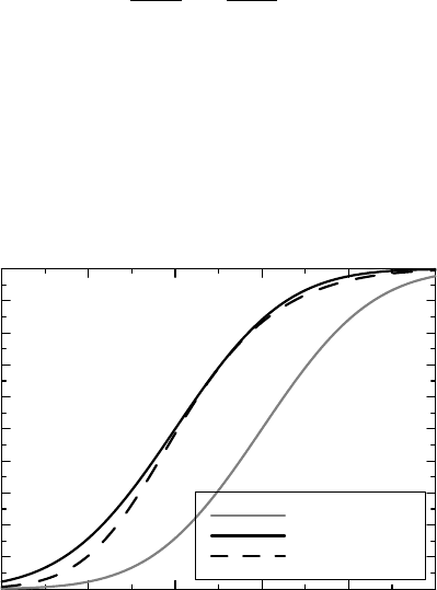
Figure 8.2 illustrates what the function G(x) looks like when it is obtained from F (x)

as described by some of these models. We start with the standard normal F (x) = (x), the

0.1

0.2

0.3

0.4

0.5

0.6

0.7

0.8

0.9

−3 −2 −1 210

Original function

Horizontal shift

Proportional odds

Figure 8.2 Illustration of how some one-parameter models change the location and shape

of the CDF. The gray curve shows the original function F (x).

212 HOW TO COMPARE THE OUTCOME IN TWO GROUPS

gray curve, which we ﬁrst shift one step to the left (we take G(x) = (x + 1)), which is the

solid black curve. The dashed curve is the CDF from the proportional odds model with factor

θ = 5. We see that both these curves are to the left of the original, and that the proportional

odds model has also changed the shape of the CDF.

We will use the following notation in this chapter. The sample taken from F(x) is denoted

by x

,...,x

and that from G(x) is denoted by y

,...,y

. Combining these two samples

gives a sample from a population whose CDF is given by

(x) = rF (x) + (1 − r)G(x).

Here r is the probability that a randomly chosen individual is from the ﬁrst group. If we have

two real groups, such as men and women, it is the fraction of the ﬁrst group within the total,

whereas in a randomized clinical trial situation, r is deﬁned by the allocation ratio to the two

groups. With a balanced randomization we have r = 1/2. The samples from the two groups

deﬁne two e-CDFs, F

(x) and G

(x) respectively, and the e-CDF for the total sample is



(x) =

n + m

(x) +

n + m

(x).

Note that the assumption that this is an estimate of (x) rests on the assumption that the

sample sizes actually reﬂect the underlying fraction r. Note also that the rank of a particular

observation x in the combined sample is given by

(x) = nF

(x) +mG

(x);

in other words, 

(x) = R

(x)/(n + m). In a randomized study we usually make all statisti-

cal analysis conditionally on the randomization outcome, in which case we take r = n/(n + m)

in the deﬁnition of (x).

8.3 Comparison done the horizontal way

We will now discuss how we can compare the distributions F (x) and G(x) horizontally – how

to describe the difference between the two CDFs in terms of location measures. The most

important of these location measures are certain percentiles, in particular the median, together

with the mean, and the discussion is closely related to the discussion on understanding a single

CDF in Section 6.5.

We start with the mean. If the two distributions have means and standard deviations

(μ

,σ

) and (μ

,σ

), respectively, the CLT tells us that

Y −

X ∈ AsN



,



with  = μ

− μ

. To be a true horizontal shift, we need to have equal variances σ

, and

then we have that



n + m

(

Y −

X − ) ∈ AsN(0,σ

COMPARISON DONE THE HORIZONTAL WAY 213

Box 8.1 Correlation of an outcome with a group variable

It is of some interest to understand what correlation measures turn into when we correlate

an outcome variable Y with a group variable X. For this we need numerical values

for the group variable, and for convenience we choose X = 1 for the ﬁrst group and

X =−1 for the second. Let the fraction from the ﬁrst group be r, so that the mean

value of X is 2r − 1. With this notation we have that P (Y ≤ y|X = 1) = F (y) and

P(Y ≤ y|X =−1) = G(y), and the covariance is



ydF (y)(1 − (2r − 1))r +



ydG(y)(−1 − (2r − 1))(1 −r) = 2r(1 − r)(m

− m

The Pearson correlation coefﬁcient is therefore half the mean difference normalized to

the standard deviation of Y in the whole sample, since V (X) = 4r(1 − r).

In order to compute Kendall’s tau deﬁned in Box 7.1, we need to compute the prob-

ability of events of the form (Y

− Y

)(X

− X

) > 0, a criterion we see is equivalent

to the outcome variable being larger for a subject from group 1 than for group 2. This

means that if we sample one subject from each group and let Z

be the outcome for

group i, then

τ = P(Z

) − P(Z

This relates Kendall’s tau to the important non-parametric Wilcoxon test as discussed

in the main text. If we have more than one group, ordered in some way (e.g., according

to which dose of a drug a particular group is given), Kendall’s tau leads us to a related

non-parametric test, the Jonckheere–Terpstra test, which is sometimes used to establish

dose response.

This actually reduces this discussion to the results obtained for the one-sample t-test in

Section 6.5. All we need is an estimate of σ

, for which we use the pooled sample vari-

ance deﬁned by

(n − 1)s

+ (m − 1)s

n + m − 2

which leads us to the approximate conﬁdence function

C() = 



 − (¯y − ¯x)

√

1/n + 1/m



If our original data are actually described by shifted Gaussian distributions, we obtain exact

inference if we replace (x) with the CDF for the t(n + m − 2) distribution, because under

that assumption the numerator of s

is a sum of two independent χ

distributions with n − 1

and m − 1 degrees of freedom, respectively. As for the single mean parameter, the Bayesian

approach to these data allows us to view C() as a posterior probability function, with

carefully chosen (non-probabilistic) priors for the parameters (the same as in Section 6.5). We

can also use this observation to derive the a posteriori density distribution from an informative

214 HOW TO COMPARE THE OUTCOME IN TWO GROUPS

Box 8.2 Analysis of a percentile difference for two groups

Here we outline how we can obtain conﬁdence claims for the difference for a particular

percentile for two independent distributions F (x) and G(x). Consider any particular

percentile, x

,ofF (x) (so that F (x

) = p). Let the corresponding percentile for G(x)

be written x

+ θ, so that G(x

+ θ) = p. In order to obtain knowledge about θ we use

the approximation

) − p)

V (F

))

∈ χ

(1), where V (F

)) = p(1 − p)/n,

for F (x), and similarly for G(x). Since the test statistics for F(x

) and G(x

+ θ) are

independent, we can sum two quadratic forms to get

) − p)

V (F

))

+ θ) − p)

V (G

+ θ))

∈ χ

(2).

From this we derive a conﬁdence function for (x

,θ), and in order to obtain knowledge

about θ we now proﬁle x

out of this, as in Section 7.7. This means that for given θ

we estimate x

= x

(θ) by minimization, which gives us a function P

(θ)ofθ alone.

The end result is the two-sided conﬁdence function C(θ) = χ

(θ)), from which we

can obtain asymptotically correct knowledge about θ. Properly modiﬁed, this approach

also allows us to compare the two percentiles in other ways, such as their ratio.

a priori distribution for the mean difference, but we will follow the biostatistical tradition and

not discuss this any further.

In order to apply the discussion above to the data in Figure 8.1 we estimate the group

mean values of the logarithmic data to 4.99 and 3.00, respectively, which gives us a mean

difference of 1.99 with 95% conﬁdence interval (0.80, 3.17). This is the (estimated) size of

the shift in Figure 8.1. However, to get the shift back to the original measurement scale we

back-transform by exponentiation. This gives us a ratio of geometric means for treated versus

placebo of e

−1.99

, which is 14%, with 95% conﬁdence interval (4.2, 45)%.

Next we consider the median. A key difference between the mean and the median is that

whereas the difference of two means is the mean of the difference, this need not be true for

medians. So the approach is more complicated, building on ideas used in Section 7.7 when

we analyzed two independent binomial parameters. An outline is given in Box 8.2. When

we carry out this analysis for our sputum data on the log scale, we get an estimated median

difference of 1.83 with 95% conﬁdence interval (0.26, 3.39), which we can back-transform

to a statement about the ratio of the medians for the two distributions as being 16% with 95%

conﬁdence interval (3.4, 77)%. For these data there is therefore a close agreement between

the mean and median estimates of a possible horizontal shift. The conﬁdence interval for the

median is wider than that for the mean, because the mean value analysis uses more of the

information in the data than the median analysis does.

Now we return to the original cell count scale, instead of their log values. For the mean

values we have the estimates 752 and 93 for the two groups, giving a mean difference estimate

of 659 with 95% conﬁdence interval (−34, 1351). In this computation we have assumed equal

COMPARISON DONE THE HORIZONTAL WAY 215

0.1

0.2

0.3

0.4

0.5

0.6

0.7

0.8

0.9

Fraction ofpatients

10008006004002000

Neutrophil count/

sputum

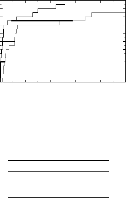
Figure 8.3 The percentile difference increases with level for the sputum data on the

original scale.

standard deviations and used the t distribution. But the standard deviations are estimated as

1521 and 157 respectively, so it is probably not a valid assumption to make. Alternatively, we

can analyze the difference for some percentiles, as described in Box 8.2. The result for the

median and the two quartiles is shown in the following table:

Parameter Estimate 95% CI

25% −33.5(−69, −8)

50% −96.5(−459, −14)

75% −485 (−4260, 312)

Figure 8.3 shows the percentile differences as horizontal lines connecting the corresponding

percentiles for the two e-CDFs. Clearly the differences vary considerably between levels,

strongly indicating that it is not appropriate to assume that the two distributions are simple

shifts of each other.

A little mathematics explains this observation. For two Gaussian distributions N(μ

,σ

)

and N(μ

,σ

), the percentile difference is given by

= μ

− μ

+ (σ

− σ

where z

is the pth percentile for the standardized Gaussian distribution. In particular, this

shows that we have a horizontal shift precisely when the variances are equal; only then is

independent of p. For lognormal distributions we have the percentiles x

= e

μ+σz

, and

when we have equal σ, the percentile difference becomes

= e

+σz

− e

+σz

= e

σz

− e

which increases with p if μ

/= μ

. This is, to a reasonable approximation, what happens in

our data.

216 HOW TO COMPARE THE OUTCOME IN TWO GROUPS

8.4 Analysis done the vertical way

This section is about the famous Wilcoxon two-group test, which may come as a surprise,

since a casual look at the following pages shows a considerable number of mathematical

expressions involving integrals. The Wilcoxon test is usually presented as a very simple test:

rank-transform data and do a few simple calculations. However, the framework within which

we derive it has a number of important extensions built into it. It becomes more than a simple

test for equality; it also provides a method to do parameter estimation. The price for this is a

little more mathematics.

The vertical approach for comparing two independent CDFs F (x) and G(x) looks for a

vertical shift (x) = F (x) − G(x) of the two CDFs at different points x. In this section we

will tacitly assume that the true CDFs are both continuous, a restriction that will be removed

in Section 8.6. Essentially there are two major ways to derive scalar quantities from (x) that

we can use to test the null hypothesis that (x) = 0 for all x. The obvious way may be to look

for the maximal difference, which we estimate by

= max

(x) −G

(x)|.

This leads us to the Kolmogorov–Smirnov test, which is discussed in Appendix 6.A.2. Al-

ternatively we may take a weighted average



∞

−∞

(x)dw(x)ofthe(x) with some weight

function w(x). A partial integration and some algebra shows that this is proportional to



∞

−∞

w(x)d(F (x) − (x)), (8.4)

which is the integral we want to concentrate on. It is zero if the distributions are equal, whatever

weights we choose. We typically want to take the weights where the data are, and one way to

ensure this is to use a function of the CDF for the combined sample, so that w(x) = a((x)).

This means that the requirement for the integral to be zero is that



∞

−∞

a((x))dF (x) =



a(u)du,

where we have changed to the variable u = (x) in the integral



a()d (we consider only

continuous distributions at present). The corresponding test statistic is obtained if we insert

e-CDFs instead of the CDFs:



∞

−∞

a(

(x))dF

(x).

We can use this to test the hypothesis of equality and also to estimate a parameter in some

simple models. We will illustrate this in some detail by looking closely at the simplest choice of

weight function, which is to take a(u) = u, so that w(x) = (x). This gives us the test statistic



∞

−∞

(x)

n + m

(x) =

n(n + m)



i=1

so this test amounts to the analysis of the total rank sum of the ﬁrst sample and is the well-known

Wilcoxon rank sum statistic. Under the null hypothesis F (x) = G(x), the expected value of the

rank sum is n(n + m + 1)/2, so we test the null hypothesis of equality by comparing the rank

ANALYSIS DONE THE VERTICAL WAY 217

Box 8.3 The Wilcoxon test and the rank-transformed t-test

To compute the p-value for the Wilcoxon test based on the statistic W =



R(x

), we

ﬁrst compute its mean and variance under the null hypothesis (we assume no ties):

E(W) =

n(N + 1)

,V(W) =

nm(N + 1)

where N = n + m. Appealing to large-sample theory, we can show that

T =

W − E(W)

√

V (W )

∈ AsN(0, 1),

from which p-values can be computed.

This is closely related to the following procedure: ﬁrst rank-transform all the data

and then apply the t-test to the resulting data. For this test the mean difference and

pooled sample variance are given by



W −

n(N + 1)



and s

(N − 2)nm

V (W )(N − 1 − T

respectively. The corresponding t-statistic is therefore given by





1 +

1−T

N−2

This relationship holds also in the presence of ties, and shows that for all practical

purposes we can compute the Wilcoxon test by applying the t-test to rank-transformed

data, at least when the sample size is large enough to allow for the asymptotic p-values

(conventionally considered to be when N ≥ 40).

There is also a relation to the Wilcoxon probability P

. In fact, the relation between

Mann–Whitney scores and the rank sum discussed in the text shows that the true mean

difference is 

= N(P

− 1/2). We can therefore use the information obtained from

the t-test on ranks to obtain an estimate and approximate conﬁdence interval for P

when the sample is large.

sum to this value. This test is frequently used in biostatistics as an alternative to Student’s t-test

to compare two independent distributions when data are distinctly non-Gaussian in nature.

The Wilcoxon rank sum test is sometimes referred to as a test of medians, which it is not. It

is a test of the mean rank and has no more to do with medians than the t-test has. In fact, it

is essentially a t-test on the ranks of the observations, instead of the original observations, as

outlined in Box 8.3. To put it another way, we apply the t-test to the variable (X) instead

of X (which is a non-linear transformation of data), a variable which we know has a uniform

distribution on (0, 1) when the null hypothesis of equal distributions for the two groups holds.

When it comes to computing p-values for the Wilcoxon test, this can be done in different

ways, which we will discuss in the next section. For the rest of this section we will instead try

to better understand the nature of the test. It is to a large extent a mathematical investigation

of relationships and is about how we transform the test into a parameter estimation method.

218 HOW TO COMPARE THE OUTCOME IN TWO GROUPS

Box 8.4 An alternative derivation of the Hodges–Lehmann estimator

An alternative derivation of equation (8.7) is based on the squared horizontal difference

between the two CDFs,



∞

−∞

(F (x) − G(x))

as the measure of the extent to which they differ. We can use this to estimate the θ in

the shift model deﬁned by equation (8.1) by considering the function

(θ) =



∞

−∞

(F (x − θ) −G(x))

dx.

For this function we have that L

(0) = L

; also, when F (x) = G(x), we have that L

(θ)

has its minimum (which is zero) when θ = 0. Therefore, if the minimum of L

(θ)is

at a point other than zero, we cannot have equality of the two distribution functions.

A short calculation shows that θ is the point where L

(θ) is minimal precisely when

equation (8.7) is fulﬁlled.

This characterization of the Hodges–Lehmann estimator suggests various related

parameters obtained by minimizing the integral



∞

−∞

w(x)(F (x − θ) − G(x))

as a function of θ, for some speciﬁed weight function, preferably of the form

w(x) = a((x)).

We have seen that the Wilcoxon test is derived from the relationship



∞

−∞

F (x)dF (x) =

, (8.5)

which is true for every continuous CDF F (x). This statement says that the mean value of

F (X)is1/2, when F (x) is the CDF for the stochastic variable X. When G(x) = F (x) there

are a few equivalent statements, including



∞

−∞

G(x)dF (x) =



∞

−∞

(x)dF (x) =



∞

−∞

(x)d(x) =

For each of these integrals there is a test statistic obtained by replacing the CDFs with

e-CDFs, and each such test statistic will provide the Wilcoxon test. We will pick the ﬁrst

of these, because this will simplify variance computation. We will also generalize it, so that

we let the function G(x) depend on a single parameter θ, which we write G(x, θ). Providing

evidence that the equation



∞

−∞

G(x, θ)dF(x) =

(8.6)

does not hold then constitutes evidence against the null hypothesis that G(x, θ) = F (x). More

importantly, we can use this equation to estimate and obtain knowledge of θ.

ANALYSIS DONE THE VERTICAL WAY 219

The classical example of parameter estimation here is when we do it on the shift model

G(x) = F (x − θ). We then have that F(x) = G(x + θ), and the θ we require is the parameter

value that solves the equation



∞

−∞

G(x + θ)dF (x) =

. (8.7)

This equation means that θ is the median of the CDF

H(z) =



∞

−∞

G(x + z)dF (x) =



y−x≤z

dF (x)dG(y).

This is the CDF for the stochastic variable Z = Y − X, where X and Y are independent with

CDFs F (x) and G(x), respectively. When F(x) = G(x) we have that H(0) = 1/2, where H(0)

is the probability P(Y<X) that Y is less than X, which we call the Wilcoxon probability and

denote by P

. This parameter must be clearly distinguished from the p-value obtained from

an application of the Wilcoxon test to test the null hypothesis.

From this discussion we can immediately derive two ways to disprove the null hypothesis

that G(x) = F (x). We can either prove that the median θ of H(z) is not zero, or that the

Wilcoxon probability



∞

−∞

G(x)dF (x)

is not 1/2. Whichever method we use, we need to estimate H(z). For this we replace the CDFs

with the corresponding e-CDFs and obtain the estimate

(z) =



∞

−∞

(x + z)dF

(x).

This is a sum, and if we expand it we ﬁnd that it can be written as

(z) =



(z + x

) =



i,j

I(y

− x

≤ z),

so this function is obtained as the e-CDF for all the nm differences z

= y

− x

. The sample

median of H

(z) is called the Hodges–Lehmann estimate of location. It therefore serves the

same purpose of separating two distributions as the mean or median group difference. Also

note that H

(0), which estimates P

, can be written as H

(0) = U

/mn, where U

called the Mann–Whitney statistic and is deﬁned as



(1 + Z

), where Z



1ify

−1ify

The Z

are called the Mann–Whitney scores, and we may note that the sum of these, divided

by the product nm, estimates the relative difference

RD = P(Y>X) − P (Y<X) = 2P

− 1.

This is a transformation of the Wilcoxon probability that relates the comparison of continuous

data for two groups to the corresponding description of binary data. It also relates the Wilcoxon

220 HOW TO COMPARE THE OUTCOME IN TWO GROUPS

0.1

0.2

0.3

0.4

0.5

0.6

0.7

0.8

0.9

Fraction of patients

−3 −2 −1 876543210

Neutrophil count/g sputum

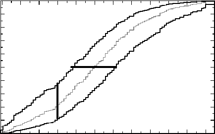
Figure 8.4 The e-CDF for the treatment difference together with pointwise conﬁdence

limits, also showing estimates and conﬁdence limits for the Hodges–Lehmann estimate (hor-

izontal line) of location and the Wilcoxon probability (vertical line).

probability to Kendall’s τ (see Box 8.1). Note further that, for continuous data, the odds

/(1 − P

) can be interpreted as an odds ratio comparing the two groups, (see page 127; this

is the generalized odds mentioned in Box 7.1). If we compare Gaussian variables with a mean

difference  and a common variance σ

, this log-odds ratio is essentially proportional to the

standardized difference /σ. (This can be seen by approximating the Gaussian distribution

with a logistic one; see Box 9.4.) Finally, the Mann–Whitney statistic is equivalent to the

Wilcoxon rank sum, because n(n + 1)/2 + U

is equal to



∞

−∞

(x)dF

(x) +nm



∞

−∞

(x)dF

(x) = n



∞

−∞

(x)dF

(x),

where the right-hand side is the rank sum of the ﬁrst group.

Figure 8.4 shows the function H

(z) for the logarithm of the sputum cell count data

as the gray staircase function in the middle. It is surrounded by pointwise 95% conﬁdence

limits, such that for a given z, the vertical interval determined by the black curves deﬁnes

the pointwise conﬁdence interval for H (z). How these conﬁdence limits are calculated will

be discussed below. In the graph there are also two conﬁdence intervals shown as solid lines:

the horizontal one at the level 1/2 shows that of the Hodges–Lehmann estimator, which is

estimated as 1.97 with 95% conﬁdence interval (0.74, 3.15). The vertical line represents a

conﬁdence interval for the Wilcoxon probability P

for which we have the estimate 0.22

with 95% conﬁdence interval (0.11, 0.38). Both conﬁdence intervals convey proof, at the

conventional two-sided 5% signiﬁcance level, of a treatment effect – the ﬁrst excludes 0 and

the second excludes 1/2.

We have tacitly analyzed the log-count of the sputum data. If we choose to analyze the

count directly, the only thing that changes is the shape of H

(z) and the Hodges–Lehmann

estimate. The Wilcoxon test and the Wilcoxon probability are both independent of the scale

on which we analyze the data. On the original scale we obtain a Hodges–Lehmann location

estimate of 60 with 95% conﬁdence interval (19, 129). This is the median of the differences, as

opposed to the difference in medians which was analyzed earlier. The estimate 1.97 discussed