Kazuaki Taira. Boundary Value Problems and Markov Processes

Подождите немного. Документ загружается.

1 Introduction and Main Results 5

(i) For every positive number ε, there exists a positive constant r

(ε) such

that the resolvent set of A

contains the set

(ε)=



λ = r

iθ

: r ≥ r

(ε), −π + ε ≤ θ ≤ π − ε



and that the resolvent (A

− λI)

−1

satisﬁes the estimate



− λI)

−1



≤

(ε)

|λ|

for all λ ∈ Σ

(ε), (1.4)

where c

(ε) is a positive constant depending on ε.

(ii) The operator A

generates a semigroup U

on the space L

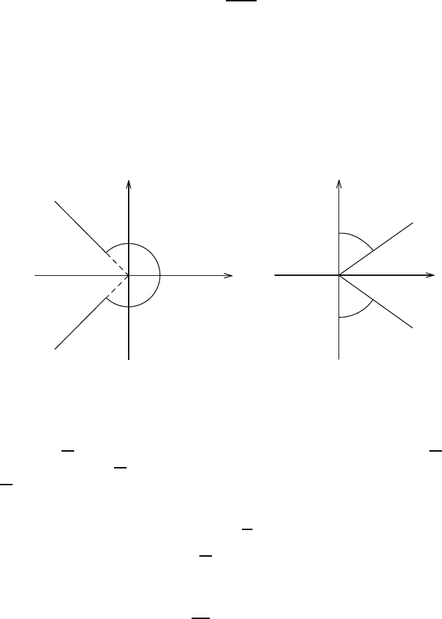
(D) which is

analytic in the sector

= {z = t + is : z =0, |arg z| <π/2 − ε}

for any 0 <ε<π/2 (see Figure 1.2).

(ε)

⏐λ⏐

(ε)

Fig. 1.2.

Secondly, we state a generation theorem of analytic semigroups in the

topology of uniform convergence.

Let C(

D) be the space of real-valued, continuous functions f(x)onD.We

equip the space C(

D) with the topology of uniform convergence on the whole

D; hence it is a Banach space with the maximum norm

f

∞

=max

x∈D

|f(x)|.

We introduce a subspace of C(

D) which is associated with the boundary

condition L. We remark that the boundary condition

Lu = μ(x



)

∂u

∂n

+ γ(x



)u =0 on∂D

6 1 Introduction and Main Results

includes the condition

u =0 onM = {x



∈ ∂D : μ(x



)=0},

if γ(x



) =0onM . With this fact in mind, we let

(D \ M )=



u ∈ C(D):u =0onM



The space C

(D\M) is a closed subspace of C(D); hence it is a Banach space.

Furthermore, we introduce a unbounded linear operator A from C

(D \ M)

into itself as follows:

(a) The domain of deﬁnition D(A)ofA is the set

D(A )=



u ∈ C

(D \ M ):Au ∈ C

(D \ M ),Lu=0



. (1.5)

(b) Au = Au, u ∈D(A).

Here Au and Lu are taken in the sense of distributions (see Chapter 9).

Then Theorem 1.2 remains valid with L

(D)andA

replaced by C

(D\M)

and A, respectively. More precisely, we can prove the following:

Theorem 1.3. Assume that condition (A) and the following condition (B



)

(replacing condition (B)) are satisﬁed:



) γ(x



) ≤ 0 on ∂D and γ(x



) < 0 on M = {x



∈ ∂D : μ(x



)=0}.

Then we have the following two assertions:

(i) For every positive number ε, there exists a positive constant r(ε) such that

the resolvent set of A contains the set

Σ(ε)=



λ = r

iθ

: r ≥ r(ε), −π + ε ≤ θ ≤ π − ε



and that the resolvent (A − λI)

−1

satisﬁes the estimate

(A − λI)

−1

≤

c(ε)

|λ|

for all λ ∈ Σ(ε), (1.6)

where c(ε) is a positive constant depending on ε.

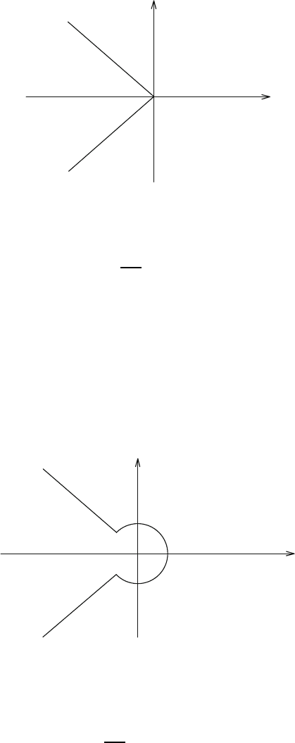
(ii) The operator A generates a semigroup T

on the space C

(D \ M) which

is analytic in the sector

= {z = t + is : z =0, |arg z| <π/2 − ε}

for any 0 <ε<π/2 (see Figure 1.3).

Moreover, the operators T

(t ≥ 0) are non-negative and contractive on

the space C

(D \M):

f ∈ C

(D \ M), 0 ≤ f(x) ≤ 1 on D \ M =⇒ 0 ≤ T

f(x) ≤ 1 on D \ M.

1 Introduction and Main Results 7

Σ (ε )

⏐λ⏐

= r(ε)

Fig. 1.3.

The main purpose of this book is devoted to the functional analytic ap-

proach to the problem of existence of Markov processes in probability theory.

A strongly continuous, non-negative and contraction semigroup {T

}

t≥0

on the space C

(D \ M) is called a Feller semigroup on D \ M.

Therefore, we can reformulate part (ii) of Theorem 1.3 as follows:

Theorem 1.4. Assume that conditions (A) and (B



) are satisﬁed. Then the

operator A generates a Feller semigroup {T

}

t≥0

on the space D \ M .

Theorem 1.4 generalizes Bony–Courr`ege–Priouret [BCP, Th´eor`eme XIX]

to the case where μ(x



) ≥ 0 on the boundary ∂D (cf. [Ta2, Theorem 10.1.3]).

It is known (cf. [Dy2], [Ta2, Chapter 9]) that if {T

}

t≥0

is a Feller semigroup

D \ M , then there exists a unique Markov transition function p

(x, ·)on

the space

D \ M such that

f(x)=



D\M

(x, dy)f(y),f∈ C

(D \ M ).

Furthermore, it can be shown that the function p

(x, ·) is the transition func-

tion of some strong Markov process X; hence the value p

(x, E) expresses the

transition probability that a Markovian particle starting at position x will be

found in the set E at time t.

The diﬀerential operator A describes analytically a strong Markov pro-

cess with continuous paths in the interior D such as Brownian motion (see

Figure 1.4).

The terms μ(x



)∂u/∂n and γ(x



)u of the boundary condition L are sup-

posed to correspond to reﬂection and absorption phenomena, respectively.

The situation may be represented schematically by Figure 1.5.

Hence the intuitive meaning of condition (B



) is that absorption phe-

nomenon occurs at each point of the set M = {x



∈ ∂D : μ(x



)=0}, while

reﬂection phenomenon occurs at each point of the set ∂D \ M = {x



∈ ∂D :

μ(x



) > 0}. In other words, a Markovian particle moves in the space D \ M

8 1 Introduction and Main Results

∂D

Fig. 1.4.

∂D

absorption reﬂection

Fig. 1.5.

until it “dies” at the time when it reaches the set M where the particle is

deﬁnitely absorbed (see Figure1.6). Therefore, Theorem 1.4 asserts that there

exists a Feller semigroup corresponding to such a diﬀusion phenomenon.

M = {¹ =0}

∂D

Fig. 1.6.

It is worth while pointing out here that the condition

μ(x



) ≥ 0andγ(x



) ≤ 0on∂D

is necessary in order that the operator A is the inﬁnitesimal generator of a

Feller semigroup {T

}

t≥0

on D \ M (cf. [Ta2, Section 9.5]).

1 Introduction and Main Results 9

As an application of Theorem 1.2, we consider the following semilinear

initial-boundary value problem: Given functions f (x, t, u, ξ)andu

(x) deﬁned

in D×[0,T)×R×R

and in D, respectively, ﬁnd a function u(x, t)inD×[0,T)

such that

⎧

⎨

⎩



∂

∂t

− A



u(x, t)=f (x, t, u, grad u)inD × (0,T),

Lu(x



,t)=μ(x



)

∂u

∂n

+ γ(x



)u =0 on∂D × [0,T),

u(x, 0) = u

(x)inD.

(1.7)

By making use of the operator A

, we can formulate problem (1.7) in terms

of the abstract Cauchy problem in the Banach space L

(D) as follows:



= A

u(t)+F (t, u(t)) , 0 <t<T,

t=0

= u

(1.8)

Here u(t)=u(·,t)andF (t, u(t)) = f (·,t,u(t), grad u(t)) are functions deﬁned

on the interval [0,T), taking values in the space L

(D).

We can prove local existence and uniqueness theorems for problem (1.8)

(Theorems 10.1 and 10.2), by using the theory of fractional powers of analytic

semigroups. Our semigroup approach here can be traced back to the pioneering

work of Fujita–Kato [FK] on the Navier–Stokes equation in ﬂuid dynamics.

Theorem 1.5. Assume that conditions (A) and (B) are satisﬁed. If the non-

linear term f(x, t, u, ξ) is a locally Lipschitz continuous function with respect

to all its variables (x, t, u, ξ) ∈ D ×[0,T)×R ×R

with the possible exception

of the x variables, then we have the following two assertions:

(i) If N<p<∞, then, for every function u

(x) of D(A

), problem (1.8) has

a unique local solution u(x, t) ∈ C ([0,T

]; L

(D)) ∩ C

((0,T

); L

(D))

where T

= T

(p, u

) is a positive constant.

(ii) If N/2 <p<N, we assume that there exist a non-negative continuous

function ρ(t, r) on R × R and a constant 1 ≤ γ<N/(N − p) such that

the following four conditions are satisﬁed:

(a) |f(x, t, u, ξ)|≤ρ(t, |u|)(1 + |ξ|

(b) |f(x, t, u, ξ) − f (x, s, u, ξ)|≤ρ(t, |u|)(1+|ξ|

) |t − s|.



1+|ξ|

γ−1

+ |η|

γ−1



|ξ − η|.

(d) |f(x, t, u, ξ) − f (x, t, v, ξ)|≤ρ(t, |u| + |v|)(1+|ξ|

) |u − v|.

Then, for every function u

(x) of D(A

), problem (1.8) has a unique

local solution u(x, t) ∈ C ([0,T

]; L

(D)) ∩C

((0,T

); L

(D)) where T

(p, u

) is a positive constant.

Here C ([0,T]; L

(D)) denotes the space of continuous functions on the closed

interval [0,T] taking values in L

(D), and C

((0,T); L

(D)) denotes the

space of continuously diﬀerentiable functions on the open interval (0,T)taking

values in L

(D), respectively.

The rest of this monograph is organized as follows.

10 1 Introduction and Main Results

Chapter 2 is devoted to a review of standard topics from the theory of semi-

groups. Section 2.1 provides a brief description of the basic results about ana-

lytic semigroups (Theorem 2.2) which forms a functional analytic background

for the proof of Theorems 1.2 and 1.3. Moreover, Subsection 2.1.3 is devoted

to the semigroup approach to a class of initial-boundary value problems for

semilinear parabolic diﬀerential equations. By making use of fractional powers

of analytic semigroups, we formulate a local existence and uniqueness theorem

for semilinear initial-boundary value problems (Theorem 2.8).

On the other hand, Section 2.2 provides a brief description of basic deﬁ-

nitions and results about Markov processes and Feller semigroups. In Subsec-

tion 2.2.6 we prove various generation theorems of Feller semigroups by using

the Hille–Yosida theory of semigroups (Theorems 2.16 and 2.18) which form

a functional analytic background for the proof of Theorem 1.4.

In Chapter 3 we present a brief description of the basic concepts and results

of the L

theory of pseudo-diﬀerential operators which may be considered as a

modern theory of the classical potential theory. In particular, we formulate the

Besov space boundedness theorem due to Bourdaud [Bo] (Theorem 3.15) and

a useful criterion for hypoellipticity due to H¨ormander [Ho2] (Theorem 3.16)

which play an essential role in the proof of our main results.

In Chapter 4 we study the boundary value problem (1.1) in the framework

of Sobolev spaces of L

type, by using the L

theory of pseudo-diﬀerential

operators. The idea of our approach is stated as follows:

First, we consider the following Neumann problem:



(A −λ)v = f in D,

∂v

∂n

=0 on∂D.

(1.9)

The existence and uniqueness theorem for problem (1.9) is well established in

the framework of Sobolev spaces of L

type (cf. Agmon–Douglis–Nirenberg

[ADN]). We let

v = G

(λ)f.

The operator G

(λ) is the Green operator for the Neumann problem. Then

it follows that a function u(x) is a solution of problem (1.1) if and only if the

function w(x)=u(x) − v(x) is a solution of the problem



(A −λ)w =0 inD,

Lw = −Lv = −μ(x



)

∂v

∂n

− γ(x



)v = −γ(x



)v on ∂D.

However, we know that every solution w of the homogeneous equation

(A −λ)w =0 inD

can be expressed by means of a single layer potential as follows:

w = P (λ)ψ.

1 Introduction and Main Results 11

The operator P (λ) is the Poisson operator for the Dirichlet problem. Thus,

by using the operators G

(λ)andP (λ) we can reduce the study of problem

(1.1) to that of the equation

T (λ)ψ = LP (λ)ψ = −γ(x



)v, v = G

(λ)f.

This is a generalization of the classical Fredholm integral equation.

Itiswellknown(cf.[Ho1],[Ho3],[Se2],[Ty])thattheoperatorT (λ)=

LP (λ) is a pseudo-diﬀerential operator of ﬁrst order on the boundary ∂D.We

can prove that the aprioriestimate (1.2) of Theorem 1.1 is entirely equivalent

to the corresponding aprioriestimate for the operator T (λ) (Theorem 4.10).

Chapter 5 is devoted to the proof of Theorem 1.1. We study the pseudo-

diﬀerential operator T (λ) in question, and prove that conditions (A) and (B)

are suﬃcient for the validity of the aprioriestimate (1.2) (Lemma 5.1). More

precisely, we construct a parametrix S(λ)forT (λ)intheH¨ormander class

1,1/2

(∂D) (Lemma 5.2), and then apply a Besov space boundedness theorem

(Theorem 3.15) to the parametrix S(λ) to obtain the aprioriestimate (1.2)

for problem (1.1).

Here it should be emphasized that if we use instead of the Neumann prob-

lem (1.9) the Dirichlet problem as usual, then we have the following apriori

estimate for problem (1.1):

u

1,p

≤ C(λ)



f

+ |ϕ|

1−1/p,p

+ u



In other words, we can not usethisestimatetoprovethegenerationtheorem

of analytic semigroups in the L

topology.

In Chapter 6 we study the operator A

, and prove fundamental apriori

estimates for A

−λI (Theorem 6.3) which is an essential step in the proof of

Theorem 1.2. We make good use of Agmon’s method (Proposition 6.4). This

is a technique of treating a spectral parameter λ as a second-order, elliptic

diﬀerential operator of an extra variable and relating the old problem to a

new one with the additional variable.

Chapter 7 is devoted to the proof of Theorem 1.2 (Theorems 7.1 and 7.9).

Once again we make use of Agmon’s method in the proof of Theorems 7.1 and

7.9. In particular, Agmon’s method plays a fundamental role in the proof of

the surjectivity of the operator A

− λI (Proposition 7.2).

Chapter 8 and Chapter 9 are devoted to the proof of Theorem 1.3 and

Theorem 1.4. In Chapter 8 we prove part (i) of Theorem 1.3. Part (i) of

Theorem 1.3 follows from Theorem 1.2 by using Sobolev’s imbedding theorems

(Theorems 8.1 and 8.2) and a λ-dependent localization argument essentially

due to Masuda [Ma] (Lemma 8.4).

In Chapter 9 we prove Theorem 1.4 and part (ii) of Theorem 1.3. This

chapter is the heart of the subject. General existence theorems for Feller

semigroups are formulated in terms of elliptic boundary value problems with

spectral parameter (Theorem 9.12). First, we study Feller semigroups with

reﬂecting barrier (Theorem 9.14) and then, by using these Feller semigroups

12 1 Introduction and Main Results

we construct Feller semigroups corresponding to such a diﬀusion phenomenon

that either absorption or reﬂection phenomenon occurs at each point of the

boundary (Theorem 9.18). Our proof is based on the generation theorems of

Feller semigroups discussed in Section 2.2.

In Chapter 10 we study problem (1.8), and prove Theorem 1.5 by using the

theory of fractional powers of analytic semigroups (Theorems 10.1 and 10.2).

To do this, we verify that all the conditions of Theorem 2.8 are satisﬁed.

We remark that Theorem 1.5 is a generalization of Pazy [Pa, Section 8.4,

Theorems 4.4 and 4.5] to the degenerate case.

In the ﬁnal Chapter 11, as concluding remarks, we give an overview for

general results on generation theorems for Feller semigroups proved mainly

by the author using the theory of pseudo-diﬀerential operators ([Ho1], [Se1],

[Se2]) and the Calder´on–Zygmund theory of singular integral operators ([CZ]).

In Appendix A, we formulate various maximum principles for second-

order elliptic diﬀerential operators such as the weak maximum principle

(Theorem A.1) and the Hopf boundary point lemma (Lemma A.3) which

play an important role in Chapter 9.

The following diagram gives a bird’s eye view of Markov processes, Feller

semigroups and boundary value problems and how these relate to each other:

Probability Functional Partial Diﬀeren-

Analysis tial Equations

Markov process Feller semigroup inﬁnitesimal

X {T

} generator A

Markov transition T

f =



(·,dy)f(y) T

=exp[tA]

function p

(·,dy)

Chapman and semigroup property diﬀerential

Kolmogorov T

t+s

= T

· T

operator A

equation

absorption function space boundary

and reﬂection C

(D \ M ) condition L

phenomena

Semigroup Theory

This chapter is devoted to a review of standard topics from the theory of

semigroups which forms a functional analytic background for the proof of

Theorems 1.2, 1.3, 1.4 and 1.5.

2.1 Analytic Semigroups

This section provides a brief description of the basic results of the theory

of analytic semigroups which forms a functional analytic background for the

proof of Theorems 1.2 and 1.3. Moreover, Subsection 2.1.3 is devoted to the

semigroup approach to a class of initial-boundary value problems for semi-

linear parabolic diﬀerential equations (Theorem 2.8). Theorem 1.5 follows by

verifying all the conditions of Theorem 2.8. For more leisurely treatments

of analytic semigroups, the reader is referred to Friedman [Fr1], Pazy [Pa],

Tanabe [Tn], Yosida [Yo] and also Taira [Ta4].

2.1.1 Generation of Analytic Semigroups

Let E be a Banach space over the real or complex number ﬁeld, and let

A : E → E be a densely deﬁned, closed linear operator with domain D(A).

Assume that the operator A satisﬁes the following two conditions (see

Figure 2.1 below):

(1) The resolvent set of A contains the region

= {λ ∈ C : λ =0, |arg λ| <π/2+ω}, 0 <ω<π/2.

(2) For each ε>0, there exists a positive constant M

such that the resolvent

R(λ)=(A − λI)

−1

satisﬁes the estimate

R(λ)≤

|λ|

for all λ ∈ Σ

= {λ ∈ C : λ =0, |arg λ|≤π/2+ω − ε}.

(2.1)

K. Taira, Boundary Value Problems and Markov Processes,13

Lecture Notes in Mathematics 1499, DOI 10.1007/978-3-642-01677-6

 Springer-Verlag Berlin Heidelberg 2009

14 2 Semigroup Theory

Fig. 2.1.

Then we let

U(t)=−

2πi



λt

R(λ) dλ. (2.2)

Here Γ is a path in the set Σ

consisting of the following three curves (see

Figure 2.2):

(1)



−i(π/2+ω−ε)

:1≤ r<∞



(2)



iθ

: −(π/2+ω − ε) ≤ θ ≤ π/2+ω − ε



(3)



i(π/2+ω−ε)

:1≤ r<∞



(1)

(2)

(3)

Fig. 2.2.

It is easy to see that the integral

U(t)=−

2πi



k=1



(k)

λt

R(λ) dλ