Kelly J.J. Graduate Mathematical Physics, With MATHEMATICA Supplements
Подождите немного. Документ загружается.

146 5 Integral Transforms
1 0 1 2 3 4 5 6
Ω
0
tt
0.05
0
0.05
0.1
0.15
0.2
0.25
Gt,t
Γ Ω
0
2
Γ Ω
0
1
Γ Ω
0
0.5
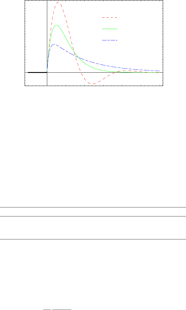
Figure 5.6. Green function for damped oscillator.
Figure 5.6 compares these functions for representative values of Γ/ Ω
0
. All are damped
exponentially but the underdamped solution also oscillates while the critically damped
and overdamped do not. The amplitude is suppressed for the overdamped oscillator, but
the duration can be long because the response is slow. Notice that SinhΚt contains expo-
nentially growing and decaying components, but that because Κ < Γ the net effect is damp-
ing with a relatively slow asymptotic form proportional to ExpΓ Κt. By contrast,
the critically-damped oscillator has a fairly strong response for a more limited duration
because the damping is sufficiently strong to suppress oscillations but weak enough to per-
mit a significant response to the impulse.
Table 5.3. Green functions for damped oscillator.
Type Condition Gt,t
'
Ω
underdamped Γ < Ω
0
Ω
1
R
ExpΓt t
'
SinΩ
R
t t
'
<t t
'
ΓΩ
R
overdamped Γ > Ω
0
Κ
1
ExpΓt t
'
SinhΚt t
'
<t t
'
ΓΚ
critically damped ΓΩ
0
ExpΓt t
'
t t
'
<t t
'
Γ
It is also of interest to consider the Green function for an ideal undamped oscillator
with Γ0. This function can be obtained by evaluating the limit Γ!0
in which the
poles for an underdamped oscillator approach the real axis from below, whereby
Γ!0
Gt,t
'
Ω
1
0
SinΩ
0
t t
'
<t t
'
(5.132)
exhibits undamped oscillations with amplitude Ω
1
0
following a unit impulse. However, if
we were to evaluate the Fourier integral
Gt,t
'
Ω
2Π
Ωtt
'
Ω
2
0
Ω
2
(5.133)

5.4 Cosine or Sine Transforms for Even or Odd Functions 147
directly, we would need a prescription for handling the poles on the real axis. In order to
obtain a physically sensible result in which effects (oscillation) follow causes (impulse),
we need to exclude the poles for t<t
'
and include them for t>t
'
. This prescription is
realized by the substitution Ω
0
!Ω
0
Γthat recognizes that any real physical system
should have a damping mechanism that will shift its resonances slightly below the real
axis and provide convergence for the delayed response of the system. Of course, we must
have Γ > 0 to ensure damping rather than spontaneous growth of small perturbations.
5.3.4 Operator Method
The differential equation for the damped oscillator can be expressed as
xt f t with
(
2
(t
2
2Γ
(
(t
Ω
2
0
(5.134)
where is a linear differential operator whose Fourier transform becomes
˜
Ω
2
2ΩΓ Ω
2
0
˜
˜x
˜
f (5.135)
The Green function represents the response to an impulse whose spectral representation is
a constant, such that
˜
˜
G 1
˜
G
˜
1
(5.136)
Therefore, a formal solution can be expressed in the form
˜xΩ ˜x
0
Ω
˜
GΩ
˜
f Ω with
˜
˜x
0
0 ,
˜
G
˜
1
(5.137)
where ˜x
0
is in the null space of the operator
˜
. The zeros of
˜
correspond to the poles of
˜
G
where
˜
0 ΩΓΩ
2
0
Γ
2
1/ 2
(5.138)
Thus, the poles of
˜
G in the complex frequency plane represent the resonances of the sys-
tem. The oscillation frequency is determined by the real part and the damping by the
imaginary part of the complex resonant frequency. Confinement of the poles to the lower
half-plane is required by causality, such that effects follow causes, and the necessity that
the effect of small perturbations decay rather than grow with time.
5.4 Cosine or Sine Transforms for Even or Odd Functions
For functions that are either even or odd with respect to reflection, such that f tf t,
it is sometimes convenient to employ Fourier cosine or sine transforms defined by
C
f t
Ω
˜
f
C
Ω
0
t CosΩt f t (5.139)
S
f t
Ω
˜
f
S
Ω
0
t SinΩt f t (5.140)

148 5 Integral Transforms
for Ω > 0. The inverse transformations are obtained with the assistance of the orthogonal-
ity relations
0
t CosΩt CosΩ
'
t
Π
2
∆Ω Ω
'
∆ΩΩ
'
(5.141)
0
t SinΩt SinΩ
'
t
Π
2
∆Ω Ω
'
∆ΩΩ
'
(5.142)
such that
f tf t f t
2
Π
0
ΩCosΩt
˜
f
C
Ω (5.143)
f tf t f t
2
Π
0
ΩSinΩt
˜
f
S
Ω (5.144)
Obviously, the relevant representation is dictated by the reflection symmetry of the original
function because the inversion of the cosine (sine) transform automatically produces an
even (odd) function of t.
The Fourier sine and cosine transforms can also be applied to generic functions with
arbitrary reflection properties, but in such cases we need both. Decomposing a generic
function into symmetric and antisymmetric components
f
t
1
2
f t f t f t f
t f
t (5.145)
with transforms
˜
f
C
Ω
0
t CosΩt f
t f
t
2
Π
0
ΩCosΩt
˜
f
C
Ω (5.146)
˜
f
S
Ω
0
t SinΩt f
t f
t
2
Π
0
ΩSinΩt
˜
f
S
Ω (5.147)
one obtains
f t
2
Π
0
Ω
˜
f
C
Ω CosΩt
˜
f
S
Ω SinΩt
(5.148)
The usual Fourier transform is then given by the combination
˜
f Ω 2
˜
f
C
Ω
˜
f
S
Ω
(5.149)
The details are left to the reader.
5.5 Discrete Fourier Transform
The continuous Fourier transform is extremely valuable for formal analysis, but often we
are left with Fourier integrals that cannot be evaluated symbolically. However, numerical
analysis using computer programs is usually limited to finite intervals and to discrete arrays

5.5 Discrete Fourier Transform 149
instead of continuous functions. Alternatively, one often samples the response of a physical
system at a set of equally spaced times and wishes to perform a spectral (Fourier) analysis
of such data. Therefore, it is of practical interest to return to the complex Fourier series
but now using a discrete time variable. The discrete Fourier transform finds innumerable
applications in the physical sciences. Among them are:
• modeling processes where the response of a system is described as convolution of a
driving force with a Green function;
• analysis of data where the desired signal is convoluted with an instrumental resolution;
• identification of periodic components using a power spectrum or an autocorrelation
function;
• suppression of noise by digital filtering.
In this section we will survey some of the technology that facilitates practical applications
of the Fourier transform to problems requiring either numerical methods or analysis of
noisy data. However, this is a very broad subject and we cannot possibly study the spe-
cialized techniques that have been optimized for various types of applications in any real
depth. Our intention here is to familiarize the student with some of the underlying princi-
ples, but the researcher will need to consult more specialized literature.
5.5.1 Sampling
It is useful to express times and frequencies as
t
j
j 1$t, j 1,N (5.150)
Ω
k
k 1$Ω ,k 1,N (5.151)
where
T N 1$t, $Ω 2Π/T (5.152)
Similarly, discretized functions become
f
j
f t
j
,
˜
f
k
˜
f Ω
k
(5.153)
and one anticipates that the discrete Fourier transform would take the form
f
j
N
k1
˜
f
k
ExpΩ
k
t
j
N
k1
˜
f
k
Exp
2Π
N
j 1k 1
(5.154)
˜
f
k
1
N
N
j1
f
j
ExpΩ
k
t
j
1
N
N
j1
f
j
Exp
2Π
N
j 1k 1
(5.155)

150 5 Integral Transforms
where we have chosen an asymmetric but convenient normalization convention for which
the first element of the transform
˜
f
1
1
N
N
j1
f
j
(5.156)
reduces to the average value of f . Note that some authors choose indices 0 j<N 1or
1
N
2
j
N
2
for even N, but we chose 1 j N because that is usually most suitable
for indexing the elements of an array within a computer program.
To verify this analogy between continuous and discrete Fourier transforms, we need to
demonstrate the discrete version of the orthogonality relation. Substitution of the Fourier
coefficients into the series gives
f
j
1
N
N
k1
N
j
'
1
f
j
'
ExpΩ
k
t
j
'
t
j
1
N
N
k1
N
j
'
1
f
j
'
Exp
2Π
N
k 1 j
'
j
(5.157)
We are free to interchange the summation order because these are finite series of finite
elements, such that
f
j
1
N
N
j
'
1
f
j
'
N
k1
z
j
'
j
k1
(5.158)
where
z
m
Exp2Πm/Nz
N
m
1 (5.159)
for integer m is one of the N
th
roots of unity. When j
'
j z
j
'
j
1, the inner
summation simply consists of N terms of unit value. When j
'
j, the inner sum is a finite
geometric series
N
k1
z
k1
m
1 z
N
m
1 z
m
B 0 (5.160)
that vanishes for any nonzero integer m that is not a multiple of N. Therefore, the summa-
tion over k yields a Kronecker delta function
1
N
N
k1
Exp
2Π
N
k 1 j
'
j
∆
j,j
'
(5.161)
that is the discrete analog of the Dirac delta function. The summation over j
'
then selects
just the term f
j
from the right-hand side, yielding an identity.
The time required for straightforward computation of the discrete Fourier transform
using the definition above scales with N
2
, but much more efficient algorithms that exploit
the periodicities of complex exponentials accomplish the same task in a time that scales
with N log
2
N. To appreciate the enormous savings realized by the so-called Fast Fourier

5.5 Discrete Fourier Transform 151
Transform (FFT), consider Table 5.4. Here the array dimensions increase by factors of 2,
the second and third columns represent the number of operations for straightforward and
optimized Fourier transforms, while the final column of ratios shows the factor by which
FFT is faster. Note that we have chosen N 2
n
on purpose – the maximum savings are
realized when N is a power of 2. The FFT for even N is still better than the straightforward
algorithm but the advantage is smaller; one should avoid odd or, even worse, prime values
of N for which FFT is no better than the standard algorithm. If your sample set is not a
power of 2, simply pad it with some extra zeros – the computational savings far outweigh
the cost in extra memory and, as we will see below, zero-padding is often useful anyway.
Table 5.4. Scaling of conventional versus fast Fourier transform with sample size.
NN
2
N log
2
N Ratio
512 262 144 4 608 57
1 024 1 048 576 10 240 102
2 048 4 194 304 22 528 186
4 096 16 777 216 49 152 341
8 192 67 108 864 106 496 630
16 384 268 435 456 229 376 1 170
32 768 1 073 741 824 491 520 2 185
The first widely disseminated FFT subroutine was developed by Cooley and Tukey
in the mid-60s and revolutionized numerical signal processing and related fields. Similar
FFT programs are now standard tools for numerical analysis and we assume that you can
find one in whatever computational environment you would use. Since FFT programs are
now so widely available that hardly anyone would consider writing his/her own anymore,
we will not discuss the details of those algorithms here. Useful discussions can be found in
books like Numerical Recipes (W. H. Press, B. P. Flannery, S. A. Teukolsky, and W. T. Vet-
terling, Cambridge University Press).
An important feature of the discrete Fourier transform is its periodicity:
˜
f
Nn
˜
f
n
f
Nn
f
n
(5.162)
However, the discrete Fourier transform is intended to be an approximation of the con-
tinuous Fourier transform that is suitable for numerical computation using computers, yet
the primary motivation for the Fourier transform was its ability to describe nonperiodic
functions. It seems that we have circled back to the Fourier series, but the Fourier series is
capable, at least in principle, of describing continuous functions f t with arbitrary accu-
racy (except at discontinuities) while the discrete Fourier transform represents sampled
quantities, f
i
, instead of continuous functions. On the other hand, arbitrary accuracy is
not really possible numerically because an infinite number of Fourier coefficients would
be needed, not to mention the inevitable truncation errors due to the finite number of bits
available to the digital representation of numbers in a computer. The discrete Fourier trans-
form represents N samples f
j
faithfully, whether they come from a smooth function or not,
except for truncation errors related to machine precision. The price is unwanted periodic-
ity and its effects upon transformations, like convolution, that require knowledge of the
152 5 Integral Transforms
0 50 100 150 200 250
Time channel
1
0
1
2
Samples
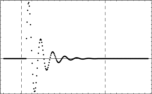
Figure 5.7. Sampling of the temporal Green function for a damped oscillator. The region within
vertical dashed lines is the working array. The exterior buffer zones contain zero-padding.
underlying physical function f t outside its sampled range. It is useful to think of f
j
as
a working array that contains sampled values f t
j
in an interior subset, l j m, with
zero-padding in buffer zones on either side, such that f
j
0for1 j<lor m< j N.
The great speed of FFT means we need not be too concerned with increasing the array size
somewhat with padding, provided that the size of the working array remains a power of 2.
This arrangement is sketched in Fig. 5.7, where the data sample the Green function for an
underdamped oscillator and where the interior and buffer zones are demarcated by dashed
vertical lines. Note that the time axis is labelled by the sample index, often called a channel.
Provided that f t is negligibly small in the outer ranges, as in this example, the artificial
periodicity induced by the discrete Fourier transform would have no adverse effects on
manipulations performed in the interior range and we would simply ignore output for the
buffer zones. We will show a practical example of this procedure in the convolution exam-
ple later. If f t does not decay fast enough when approaching the buffer zones, it might
be necessary to impose a suitable decay by hand, but the details and consequences of such
modifications vary for each case and would take us too far afield. The art of numerical
computation is as interesting, important, and challenging as the more theoretical concerns
of the present course but is beyond its scope.
For the remainder of this section we will assume that all f
j
values are real, as befitting
the sampling of a measurable quantity. The transform then exhibits the reflection symmetry

5.5 Discrete Fourier Transform 153
˜
f
Nk2
1
N
N
j1
f
j
Exp
2Π
N
j 1N k 1
1
N
N
j1
f
j
Exp
2Π
N
j 1k 1
(5.163)
such that
f f
˜
f
Nk2
˜
f
k
(5.164)
Thus, all f
j
can be reconstructed using only the first N/2 values of
˜
f
k
; the rest are redun-
dant. Has information been lost? Not really, because N/2 complex numbers still contain
N real numbers so that the transform is indeed a faithful representation of the input data.
At least two samples are needed to determine both the amplitude and the phase of any
Fourier component. On the other hand, if we think of f
j
as a discretized approximation
to a continuous real function f t, the limitation of the information content to the first half
of the spectrum means that the discrete Fourier transform cannot reproduce any temporal
variations with frequencies greater than Ω
c
Π/ $t, where $t is the sampling interval.
This maximum frequency is known as the Nyquist frequency and limits the accuracy with
which discretized representations can reproduce continuous functions. If the Fourier com-
ponents with Ω > Ω
c
are known to be negligible for our target function, then sampling
works well and calculations using discrete Fourier transforms should be limited only by
machine precision; if not, then we should reduce the sampling interval enough to achieve
the required precision. The first step in many applications is use electronic or digital filters
to suppress high-frequency components, which is especially useful when high-frequencies
contain more noise than signal.
Signals whose Fourier components are limited to Ω < Ω
max
Ω
c
are described as
bandwidth limited and are well-suited to the discrete Fourier transform. Unfortunately,
if the input signal is not bandwidth-limited, high-frequency components can distort the
lower-frequency information in the discrete Fourier transform. This phenomenon is known
as aliasing because a component with Ω/ Ω
c
n will be mistaken for contribution to
ModΩ, Ω
c
because the high-frequency wave oscillates n times between samples. This
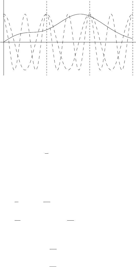
nature of this problem is illustrated schematically in Fig. 5.8. Both sinusoidal functions
have the same values at each sampled time and are thereby indistinguishable to the discrete
Fourier transform; yet they are completely different between samples.
5.5.2 Convolution
The convolution of two continuous functions is defined by
h f P g ht
f Τgt ΤΤ (5.165)
154 5 Integral Transforms
Time
Amplitude
Figure 5.8. Schematic illustration of aliasing. The solid line represents an input signal and the verti-
cal dashed lines the sampling times. Also shown are CosΩ
c
t and Cos2Ω
c
t.
where we assume that both functions vanish for t!. The convolution theorem then
tells us that the Fourier transform of a convolution
˜
hΩ
˜
f Ω˜gΩ (5.166)
is the product of the Fourier transforms of its components. Similarly, for sampled functions
we define
h f P g h
j
1
N
N
k1
f
k
g
jk1
(5.167)
where we assume that the meaningful values of sampled quantities are confined to the
interior region of suitably padded working arrays. Note the index for g
jk1
accounts for
the fact that k starts with 1 instead of 0. We now seek the discrete analog of the convolution
theorem. By direct calculation, we write
˜
h
k
1
N
N
j1
h
j
Exp
2Π
N
j 1k 1
1
N
2
N
j1
N
m1
f
m
g
jm1
Exp
2Π
N
j 1k 1
(5.168)
and substitute
f
m
N
n1
˜
f
n
Exp
2Π
N
m 1n 1
(5.169)
g
jm1
N
l1
˜g
l
Exp
2Π
N
j ml 1
(5.170)

5.5 Discrete Fourier Transform 155
to obtain
˜
h
k
1
N
2
N
j1
N
m1
N
n1
N
l1
˜
f
n
˜g
l
, Exp
2Π
N
j 1k 1m 1n 1j ml 1
(5.171)
or
˜
h
k
1
N
2
N
j1
N
m1
N
n1
N
l1
˜
f
n
˜g
l
Exp
2Π
N
j 1k lm 1n l
(5.172)
The summation over j reduces to N∆
k,l
, which then eliminates the summation over l also,
such that
˜
h
k
1
N
N
m1
N
n1
˜
f
n
˜g
k
Exp
2Π
N
m 1n k
(5.173)
Next the summation over m reduces to N∆
n,k
and we finally obtain
˜
h
k
˜
f
k
˜g
k
(5.174)
as the discrete form of the convolution theorem with the present normalization convention.
Before applying the convolution theorem to practical examples, we must consider the
effects of the offsets used to place functions comfortably within the central region of the
working array. Generally this means that the arrays are related to the underlying functions
by
f
j
f t
j
S
f
,g
j
gt
j
S
g
(5.175)
where S
f
and S
g
are somewhat arbitrary time shifts in f and g, chosen to make their sam-
pling more convenient. The continuous Fourier transforms of shifted functions
˜
f Ω
ΩS
f
f t
Ωt
t (5.176)
˜gΩ
ΩS
g
gt
Ωt
t (5.177)
include phase factors that depend upon the shifts. It is then useful to apply similar phase
shifts to the corresponding discrete Fourier transforms, whereby
˜
f
k
Exp
2Πk 1S
f
/T
N
N
j1
f t
j
Exp
2Π
N
j 1k 1
(5.178)
˜g
k
Exp2Πk 1S
g
/T
N
N
j1
gt
j
Exp
2Π
N
j 1k 1
(5.179)