Kelly J.J. Graduate Mathematical Physics, With MATHEMATICA Supplements
Подождите немного. Документ загружается.


156 5 Integral Transforms
To illustrate the use of the convolution theorem with adjustable phase shifts, consider
an underdamped harmonic oscillator with Green function Gt and driving force Ft, such
that the net displacement is given by
xt
Gt ΤFΤ Τ ˜x
˜
f ˜g (5.180)
We have already derived the Green function using the continuous Fourier transform and
found
Γ < Ω
0
Gt ΤΩ
1
R
ExpΓt ΤSinΩ
R
t Τ<t Τ,
Ω
R
Ω
2
0
Γ
2
(5.181)
Even if we know the continuous functions f t and gt, the convolution integral is usually
too difficult to perform symbolically and we need to use numerical methods. Often we do
not know the underlying functions and have only measurements made at discrete times. In
either case, let f
j
sample the force and g
j
sample the Green function. For computational
reasons we shift g
j
within the working array using zero padding on the left side, as shown
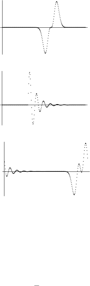
in Fig. 5.9. Suppose that the driving force is a pulse with both positive and negative lobes
centered upon t 0. This time scale is also inconvenient for numerical computation, so
we shift the sampled function into the working array. However, suppose that we were not
too clever in our choice of shift and happened to place f somewhat too far to the right, as
shown in Fig. 5.9. We then evaluate the displacement using the bare convolution theorem
without compensatory phase shifts. The bulk of the resulting function is then rather far to
the right of center and there appears to be a significant response for very early times before
the driving force even becomes active. Does the model violate causality? No, this behavior
is simply an artifact of the periodicity of the discrete Fourier transform and our injudicious
sampling choices. After all, the Green function really vanishes for negative times. By
placing it in the middle of the working array, the result of convolution is artificially shifted
to the right. With a force that is also shifted to the right, the response goes past the end
of the array and reappears, by periodicity, at the beginning. We might try placing g closer
to the left edge of the array, but that could cause other unwanted wrap-around effects for
functions that do not feature a sharp left edge.
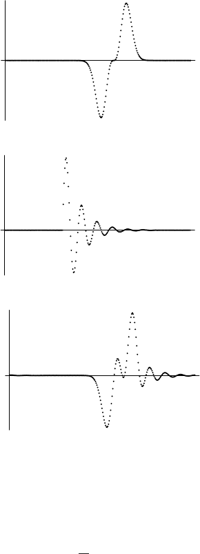
The solution to these numerical problems is to multiply
˜
f
k
˜g
k
by a phase Exp2Πk
1S
g
/T before computing the inverse Fourier transform of ˜x. This phase compensates for
the offset of g
j
and aligns the response with the driving force, as shown in Fig. 5.10. With
a larger shift, we could also compensate for the poor placement of f , but we must not
use a shift so large that it wraps around the left side and back onto the right. Because the
indexing of sampled functions is merely a computational issue, we are free to adjust it in
any manner that ensures numerical accuracy and convenience.
5.5.3 Temporal Correlation
Suppose that two functions, f t and gt, are qualitatively similar to each other, except that
there is a time shift between them. If we had graphs of those functions we could estimate
5.5 Discrete Fourier Transform 157
t
f g
t
g
t
f
Figure 5.9. Convolution without a phase shift. If either f or g is too close to the right side, periodicity
of the discrete Fourier transform produces artificial strength near the left side of their convolution,
an effect described as wrap-around.
the time shift by sliding those graphs to the left or right until we obtain the best overlap
between them. If these functions are quasiperiodic or include several features with different
periods, there may be several shifts which result in significant overlap. The correlation
function
C
j
f,g
1
N
N
k1
f
jk
g
k
(5.182)
provides a systematic method for evaluating the correlation between two sampled func-
tions. The correlation function obviously closely resembles convolution and we can deduce
˜
C
k
f,g
˜
f
k
˜g
k
(5.183)
158 5 Integral Transforms
t
f g
t
g
t
f
Figure 5.10. Convolution using a shift of 0.3125T aligns the response with the driving force and
eliminate wrap-around.
without further ado. Often one uses the autocorrelation function
C
j
f, f
1
N
N
k1
f
jk
f
k
˜
C
k
f, f
˜
f
k
2
(5.184)
to identify periodic behavior within a single time series. Thus, the Fourier transform of
the autocorrelation function is simply proportional to the spectral power distribution. If we
also employ ensemble averaging, spectral distributions in statistical physics are seen to be
closely related to probability distributions for fluctuations about equilibrium.
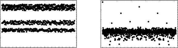
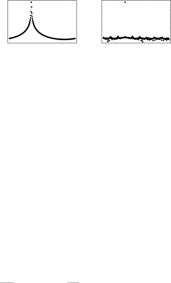
Consider the data x
k
plotted in Fig. 5.11. There appear to be three distinct bands but,
without laborious scanning of the raw data, it is not obvious to this viewer whether or
not there is additional structure within those bands or whether there is a pattern to how
the visible bands are visited. Perhaps the simplest method for studying data of this type
is to use standard mathematical software to evaluate Fourier transforms and to form the
5.5 Discrete Fourier Transform 159
0 200 400 600 800 1000
t
j
0.2
0.4
0.6
0.8
1
x
j
0 200 400 600 800 1000
Ω
k
8
6
4
2
0
Log
10
C
k
Figure 5.11. Left: noisy time series. Right: autocorrelation spectrum.
autocorrelation spectrum. This can be accomplished with only a few lines of code using
, for example. We then obtain the accompanying figure for
˜
C
j
; notice the
logarithmic scale. The strongest channel, k 1, contains the square of the sum of x
j
.
Three other strong frequencies are clearly visible, plus four weaker frequencies. Therefore,
these data actually contain an 8-cycle. (Note that alternation between two values, a 2-cycle,
only corresponds to one frequency.) In addition, there is a spectrum of white noise that
tends to obscure the patterns in x
j
.
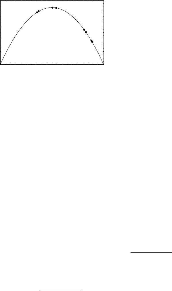
Now that we know there is an embedded 8-cycle, we can partition the data into groups
of 8 and average the groups to obtain an estimated cycle ¯x
j
,j 1, 8 for which ran-
dom fluctuations are suppressed by averaging; positive fluctuations tend to cancel negative
fluctuations. Finally, if the underlying dynamics are periodic and deterministic, the value
of x
j1
is predicted by x
j
. Therefore, Fig. 5.12 plots ¯x
j1
versus ¯x
j
for the cycle. We now
see individual points that were obscured in the noisy raw data by random fluctuations. In
a similar plot for the raw data without averaging, these pairs of points would smear out
into indistinct blobs. These points lie within the bands in the t
j
,x
j
plot, but the highest
two pairs appeared to merge into a single band in the noisy data. The lowest band was
narrowest because the underlying pair has the smallest separation. These points appear to
lie along a parabola, so we also show a curve Μx1 x where Μ is fitted to the cycle data.
The data for this simulation were constructed using the logistic map
x
j1
Μx
j
1 x
j
(5.185)
with Μ3.55, which settles onto an 8-cycle after discarding enough of the initial itera-
tions to allow transients to decay. We then added uniformly distributed random fluctuations
to simulate the noise that might be encountered in the measurement of the response of a
dynamical system. The noise amplitude was chosen to be large enough to smear the bands
in x but small enough not to obscure the smaller frequency peaks in
˜
C. The unperturbed
cycle for this Μ is actually {0.506, 0.887, 0.355, 0.813, 0.540, 0.882, 0.370, 0.828}, which
agrees well with the extracted cycle. Thus, the upper band actually contains 4 values while
the lower 2 bands contain 2 each, but it would take very sharp eyes, and perhaps some
imagination, to discern that pattern within the noisy data. Nevertheless, with the aid of the
autocorrelation spectrum we can discern the periodicities of the data and use that infor-
160 5 Integral Transforms
0.2 0.4 0.6 0.8 1
x
j
0.2
0.4
0.6
0.8
1
x
j 1
Figure 5.12. Cycle and recursion relation extracted from data in Fig. 5.11.
mation to discover the underlying dynamics despite the superimposed noise. The present
example is admittedly artificial, but it should be clear that this type of analysis can be very
valuable in the study of real dynamical systems.
5.5.4 Power Spectrum Estimation
Estimation of the power spectrum for a persistent function f t that is not localized in
time using discretely sampled measurements is a surprisingly tricky task for which there is
much lore and literature; too much to survey here. The main problem is that the limitation
of data to a finite interval necessarily sacrifices information about times outside that inter-
val. Discrete sampling also limits the maximum meaningful frequency to ΩΩ
c
Π/T
for real functions or 2Ω
c
for complex functions. Finally, there are precision and noise
issues that we will not discuss but which are important in practice. Here we will present a
very brief survey of some of the issues in estimating power spectra but leave more detailed
discussion to specialized texts.
Suppose that f tExpΩ
0
t represents a simple harmonic vibration with unique
frequency Ω
0
. Sampling necessarily limits the Fourier transform to a finite interval T .
(Who can afford to watch the vibration forever?) Thus, the continuous Fourier transform
over a finite interval becomes
˜
f Ω
T
0
ExpΩt ExpΩ
0
tt 2ExpΩΩ
0
T/2
SinΩ Ω
0
T/2
ΩΩ
0
(5.186)
with a spectral power density
PΩ
˜
f Ω
2
T
SinΩ Ω
0
T/2
Ω Ω
0
T/2
2
(5.187)
that peaks at Ω
0
but which is spread over a considerable range of frequencies when Ω
0
T
is not large. Many periods of oscillation must be observed in order to measure Ω
0
accu-

5.5 Discrete Fourier Transform 161
rately, especially when the signal contains noise or measurement errors. However, actual
measurements made are at discrete times t
j
T j 1/ N 1, not continuously, so we
estimate the power spectrum using the discrete Fourier transform
˜
f
k
N
j1
Exp
2Π
N
j 1k 1
f t
j
N
j1
Exp
2Π
N
j 1k 1 Exp
Ω
0
T
j 1
N 1
(5.188)
This expression takes the form of a finite geometric series that can be evaluated in closed
form. After some tedious algebra, we obtain
˜
f
k
Exp
Π
k 1
N
Ω
0
T
2Π
Sin
Ω
0
T
2
N
N1
Sin
Ω
0
T
2N1
Π
k1
N
(5.189)
The first factor is just a phase that does not affect the power spectrum. It is useful to define
T N 1Τ where Τ is the sampling interval, such that
P
k
SinNΩ
0
Τ/ 2
SinΩ
0
Τ/ 2 Πk 1/N
2
(5.190)
represents the discrete power spectrum. This spectrum exhibits a strong peak where
k *Κ1
Ω
0
Τ
2Π
m
N (5.191)
is close to a root of the denominator. Here m is an integer chosen to ensure that Κ is in the
range 1 ΚN. Notice that we indicated approximate equality because k is an integer
while Κ usually is not. The peak of the power spectrum then has a finite width, proportional
to T
1
, that is similar to the continuous Fourier transform of a finite wave train. When Κ
actually is an integer, both the numerator and the denominator have coincident roots and
we use L’Hôpital’s rule to determine that
NΩ
0
Τ
2Π
!ΚmN 1
˜
f
k
! N∆
k,Κ
(5.192)
is consistent with the normalization of the orthogonality relation for the discrete Fourier
transform. In principle, such a peak is limited to only one channel, but signal noise or
numerical precision will generally produce nonzero amplitudes for nearby channels.
The sensitivity of the power spectra to slight differences in frequency is illustrated in
Fig. 5.13. Both figures use FFT with N 2
8
256 channels. Notice the logarithmic
scales. The peak at Κ86.33 for Ω
0
Τ2Π/ 3 is not integral, resulting in a noticeable
spreading about channel k 86. By contrast, using the very similar frequency Ω
0
Τ
2Π/ 3N 1/Nproduces a discrete delta function at channel 86; the negligible, but appar-
ently nonzero, power in other channels is due to round-off errors for numerical calculation
162 5 Integral Transforms
0 50 100 150 200 250
k
2
1
0
1
2
Log
10
P
k
Ω
0
Τ2Π 3
0 50 100 150 200 250
k
30
25
20
15
10
5
0
Log
10
P
k
NΩ
0
Τ2Π 3N 1
Figure 5.13. Power spectra for discrete Fourier transforms of ExpΩ
0
t that use Ω
0
Τ*2Π/ 3.
of the Fourier transform with a machine precision of 10
16
. The striking difference between
these spectra is an artifact of discretization that has nothing to do with the nature of the
underlying continuous function. In one case we chose, probably fortuitously, a sampling
interval that divides the period perfectly. In real life our signals would not be pure sinusoids
and we would not know the frequency well enough in advance to choose such a precise
sampling interval – if we had such knowledge, we would not need to perform numerical
analysis. Therefore, the panel on the left is the usual situation and shows that the spectrum
is spread by sampling even for a pure sinusoidal oscillation. The panel on the right, on
the other hand, requires precise calculations and delicate cancellations to achieve a dis-
crete delta function. The alert reader might wonder how the discrete Fourier transform can
produce a delta function using a finite observation time T while the continuous Fourier
transform for the same observation time results in appreciable spread. The difference is
that the discrete Fourier transform automatically assumes that the underlying function is
periodic and persists forever while the continuous Fourier transform does not.
The term mN in the expression for Κ is a manifestation of aliasing – even when
the frequency Ω
0
is very large, there is still a peak within the sampled range of frequen-
cies because discrete sampling cannot distinguish how many times a function oscillates
between samples. Consequently, very high frequency contributions to a continuous signal
corrupt the discrete power spectrum for lower frequencies. In Fig. 5.14 we chose a fre-
quency for which Ω
0
Τ2135 is much larger than 2ΠN for N 256. The peak power for
the continuous spectrum should then be well beyond the end of this spectrum. Neverthe-
less, we observe a peak at channel 205 corresponding to m 339. Our sampling is much
too coarse to obtain a realistic spectrum for this high-frequency signal. Signal processing
cannot be performed by blind application of numerical algorithms.
As our final example, we consider the behavior of the van der Pol oscillator, described
by the differential equation
(
2
xt
(t
2
xt1 xt
2
(xt
(t
(5.193)
where is a positive constant and x will be described as a displacement. This equation
reduces to a simple harmonic oscillator when ! 0, but for positive the velocity-
dependent term pumps energy into the motion for small displacements and drains it for
5.5 Discrete Fourier Transform 163
0 50 100 150 200 250
k
2
1
0
1
2
Log
10
P
k
Figure 5.14. Power spectra for discrete Fourier transform of ExpΩ
0
t with Ω
0
Τ2135. The
peak is an artifact of aliasing; the frequency of the actual signal is much too large for this sampling
interval.
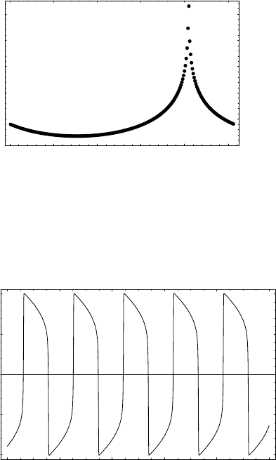
500 520 540 560 580 600
t
2
1
0
1
2
x
Figure 5.15. van der Pol oscillation, 10.
large displacements. The net effect is to drive the system toward a stable “limit-cycle”
oscillation that is decidedly nonsinusoidal for large . This nonlinear differential equation
cannot be solved symbolically, so we must resort to numerical methods. The solution for
large t, long after transients have decayed, is shown in Fig. 5.15 for 10. The behav-
ior is periodic but not simple, featuring relatively slow variations near either extreme, but
with rapid transitions between those extremes. Obviously, the time sampling must be fine
enough to represent the abrupt transitions.
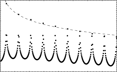
The discrete power spectrum obtained using 4096 samples in the range 200 t 600
is shown in Fig. 5.16. The peaks are found at odd multiples of a fundamental frequency, Ν
1
,
that is approximately 21 channels. The fact that the harmonics are odd can be understood
by observing that the nonlinear term responsible for those harmonics is odd. From the
plot of xt we see that the oscillation period, p, is approximately 19 time units, such that
164 5 Integral Transforms
50 100 150 200 250 300 350 400
k
2
1
0
1
2
3
4
Log
10
P
k
Figure 5.16. van der Pol spectrum, 10.
Ν
1
p * T where T is the total observation time. The dashed line shows that the intensity
of higher harmonics is roughly proportional to k
5/ 2
, at least over this range. If the time
samples represent observation of a physical system, the power spectrum can be used to
study the underlying dynamics. We might, for example, attempt to guess a differential
equation that has these features and fit its parameters to the observed behavior.
After transients have decayed away, the behavior of this system is periodic. If we knew
its functional form and period precisely, we could use the Fourier series to deduce the
power in each odd multiple of the fundamental frequency, reducing the power spectrum
from a sequence of peaks to a series of discrete spikes of zero width. The spreading seen
in the discrete Fourier transform is partly due to the limitations of sampling in which the
period is not divided into a precisely integral number of samples. We might be able to
reduce the widths of these peaks if we knew the period in advance or could interpolate
within the data array to improve the sampling interval. The mismatch between the sample
interval and the period is analogous to chopping the fundamental frequency. The sharp
turn-on at t 0 and turn-off at t T spreads each discrete frequency into a peak of
finite width. A closer approximation to a Fourier series of narrow peaks can be obtained
by multiplying the sampled data by a window function wt that has a broad, relatively flat
central region between smooth turn-on and turn-off regions. This technique is explored
in one of the end-of-chapter problems. However, in real applications, additional spreading
would be produced by measurement errors and noise. The effect of noise can be reduced by
dividing the data into several subintervals, each containing an integral number of periods,
and averaging the data for those subintervals to improve the signal-to-noise ratio. The
discrete Fourier transform would then be taken for the averaged data.

5.6 Laplace Transform 165
5.6 Laplace Transform
5.6.1 Definition and Inversion
The Laplace transform f is defined by
f t
s
˜
f s
0
t
st
f t (5.194)
and is useful for functions which vanish for t<0 and remain finite for t>0, ensuring
convergence of an integral transform that uses an exponential kernel. The Laplace trans-
form is related to the Fourier transform with respect to an imaginary variable Ω!s.The
primary difficulty in using the Laplace transform is defining and evaluating the inverse
transformation
1
. Using the analogy with the Fourier transform, we might guess that
the kernel for the inverse transform should take the form
Ωt
!
st
, but the exponential
growth for t>0 clearly presents problems for convergence. Consider the Fourier trans-
form of the function
gt
Γt
f t˜gΩ gΩ
0
t
Ωt
gt
0
t
ΓΩt
f t (5.195)
whose inverse Fourier transform satisfies
Γt
f t
1
˜g
1
2Π
Ω
Ωt
˜gΩ ft
1
2Π
Ω
ΓΩt
˜gΩ (5.196)
The integral for f t will converge if Γ is large enough to ensure that
st
gs!0fors !
. The variable change s ΓΩthen gives
f t
1
2Π
Γ
Γ
s
st
gs Γ (5.197)
where the Fourier transform of g evaluated for the imaginary frequency s Γsuch that
gs Γ
0
t
sΓt
gt
0
t
Γst
Γt
f tf s (5.198)
reduces to the Laplace transform of f . Rigorous derivations may be found in more special-
ized literature.
Therefore, the Laplace transform and its inverse are defined by
˜
f sf
0
t
st
f t (5.199)
f t
1
˜
f
1
2Π
Γ
Γ
s
st
˜
f s (5.200)
where Γ is a real number chosen to place the integration path to the right of all singularities
in
˜
f s. The inverse Laplace transform is often called the Bromwich integral or the Mellin
inversion formula. Although the Laplace transform was originally defined for real values