Klipp E., Herwig R., Kowald A., Wierling C., Lehrach H. Systems Biology in Practice: Concepts, Implementation and Application
Подождите немного. Документ загружается.


3.2.3
Solution of Linear ODE Systems
We may be interested in two different types of problems: describing the temporal
evolution of the system and finding its steady state. The problem of finding the
steady state
x of a linear ODE system
_
x = 0 implies that A
x+z= 0. The solution ne-
cessitates inversion of the system matrix A:
x A
1
z : (3-40)
The time course solution of homogeneous linear ODEs is described below. The
systems can be solved using an exponential function as approach. In the simplest
case n = 1, we have
dx
1
dt
a
11
x
1
: (3-41)
Introducing the approach x
1
(t)=b
1
e
lt
with constant b
1
into Eq. (3-41) yields:
b
1
le
lt
a
11
b
1
e
lt
: (3-42
Equation (3-42) is true if l = a
11
. This leads to the general solution
x
1
tb
1
e
a
11
t
: (3-43)
To find a particular solution, we must specify the initial conditions x
1
(t =0)=x
1
0
=
b
1
e
a
11
t
|
t=0
= b
1
. Thus, the solution is
x
1
tx
0
1
e
a
11
t
: (3-44)
For a linear homogeneous system of n differential equations,
_
x = Ax, the approach
is x = be
lt
. This gives
_
x = ble
lt
= Abe
lt
. The scalar factor e
lt
can be cancelled out,
leading to bl = Ab or the characteristic equation
A l I
n
b 0 : (3-45)
The solution of this equation is described in Section 3.1.2.
For homogeneous linear systems, the superposition principle holds: if x
1
and x
2
are solutions of this ODE system, then their linear combination is also a solution.
This leads to the general solution of the homogeneous linear ODE system:
x t
P
n
i1
c
i
b
i
e
l
i
t
; (3-46)
where b
(i)
are the eigenvectors of the system matrix A corresponding to the eigenva-
lues l
i
. A particular solution specifying the coefficients c
i
can be found considering
70
3 Mathematics in a Nutshell

the initial conditions x (t =0)=x
0
=
P
n
i1
c
i
b
i
. This constitutes an inhomogeneous
linear equation system to be solved for c
i
.
For the solution of inhomogeneous linear ODEs, the system
_
x = Ax + z can be trans-
formed into a homogeneous system by the coordination transformation
^
x = x –
x.
Since
d
dt
x = A
x+z= 0, it holds that
d
dt
^
x = A
x. Therefore, we can use the solution
algorithm for homogeneous systems for the transformed system.
3.2.4
Stability of Steady States
If a system is at steady state it should stay there, at least until an external perturba-
tion occurs. Depending on systems behavior after perturbation, their steady states
are
. stable (the system returns to this state),
. unstable (the system leaves this state), or
. metastable (the system behavior is indifferent).
A steady state is asymptotically stable if it is stable and nearby initial conditions
tend to this state for t ? ?. Local stability describes the behavior after small pertur-
bations, global stability after any perturbation.
To investigate whether a steady state
x of the ODE system
_
x = f(x) is asymptoti-
cally stable, we consider the linearized system
_
n = An (Section 3.2.1.2) with n (t)=
x(t)–
x. The steady state
x is asymptotically stable if the Jacobian A has n eigenva-
lues with strictly negative real parts each. The steady state is unstable if at least one
eigenvalue has a positive real part. This will be explained in more detail for one- and
two-dimensional systems.
We start with one-dimensional systems, i.e., n = 1. Without a loss of generality
x
1
=0orx
1
= x
1
. To the system
_
x
1
= f
1
(x
1
) belongs the linearized system
_
x
1
=
if
1
ix
1
x
1
x
1
= a
11
x
1
. The Jacobian matrix A ={a
11
} has only one eigenvalue, l
1
= a
11
=
if
1
ix
1
x
1
.
The solution is x
1
(t)=x
1
0
e
l
1
t
. It is obvious that e
l
1
t
increases for l
1
> 0 and that the
system runs away from the steady state. For l
1
< 0, the deviation from steady state
decreases and x
1
(t) ?
x
1
for t ? ?.Forl
1
= 0, consideration of the linearized system
allows no conclusion about stability of the original system.
Consider the two-dimensional case n = 2. To the system
_
x
1
f
1
x
1
; x
2
(3-47)
_
x
2
f
2
x
1
; x
2
belongs the linearized system
71
3.2 Ordinary Differential Equations
_
x
1
if
1
ix
1
x
x
1
if
1
ix
2
x
x
2
_
x
2
if
2
ix
1
x
x
1
if
2
ix
2
x
x
2
or
_
x
if
1
ix
1
x
if
1
ix
2
x
if
2
ix
1
x
if
2
ix
2
x
0
B
B
B
@
1
C
C
C
A
x
a
11
a
12
a
21
a
22
x Ax (3-48)
To find the eigenvalues of A, we have to solve the characteristic polynomial
l
2
a
11
a
22
|{z}
Trace A
l a
11
a
22
a
12
a
21
|{z}
Det A
0 (3-49)
and get
l
1=2
Trace A
2
Trace A
2
4
Det A
s
: (3-50)
The eigenvalues are either real for (Trace A)
2
/4 – Det A 6 0) or complex (other-
wise). For complex eigenvalues, the solution contains oscillatory parts.
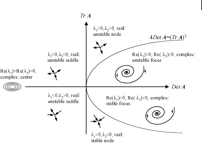
For stability it is necessary that Trace A<0 and Det A > 0. Depending on the sign
of the eigenvalues, steady states of a two-dimensional system may have the following
characteristics:
1. l
1
<0,l
2
< 0, both real: stable node;
2. l
1
>0,l
2
> 0, both real: unstable node;
3. l
1
>0,l
2
< 0, both real: saddle point, unstable;
4. Re(l
1
)<0,Re(l
2
) < 0, both complex with negative real parts: stable focus;
5. Re(l
1
)>0,Re(l
2
) > 0, both complex with positive real parts: unstable focus; or
6. Re(l
1
)=0,Re(l
2
) = 0, both complex with zero real parts: center, unstable.
Graphical representation of stability depending on trace and determinant is given
in Fig. 3.2.
Up to now we have considered only the linearized system. For the stability of the
original system, the following holds. If the steady state of the linearized system is
asymptotically stable, then the steady state of the complete system is also asymptoti-
cally stable. If the steady state of the linearized system is a saddle, an unstable node,
or an unstable focus, then the steady state of the complete system is also unstable.
This means that statements about the stability remain true, but the character of the
steady state is not necessarily kept. No statement about the center is possible.
The Routh-Hurwitz theorem (Bronstein and Semendjajew 1987) states: For sys-
tems with n > 2 differential equations, it holds that the characteristic polynomial
a
n
l
n
a
n1
l
n1
... a
1
l a
0
0 (3-51)
is a polynomial of degree n, which frequently cannot be solved analytically (at least
for n < 4). We can use the Hurwitz criterion to test whether the real parts of all eigen-
values are negative. We have to form the Hurwitz matrix H, containing the coeffi-
cients of the characteristic polynomial:
72
3 Mathematics in a Nutshell
H
a
n1
a
n3
a
n5
... 0
a
n
a
n2
a
n4
... 0
0 a
n1
a
n3
... 0
0 a
n
a
n2
... 0
.
.
.
.
.
.
.
.
.
.
.
.
.
.
.
000... a
0
0
B
B
B
B
B
B
B
@
1
C
C
C
C
C
C
C
A
fh
ik
g; (3-52)
where h
ik
follows the rule
h
ik
a
ni2k
; if 0 2k i n
0; else
: (3-53)
It can be shown that all solutions of the characteristic polynomial have negative
real parts if all coefficients a
i
of the polynomial as well as all principal leading min-
ors of H have positive values.
3.2.4.1 Global Stability of Steady States
A state is globally stable if the trajectories for all initial conditions approach it for
t ??. The stability of a steady state of an ODE system can be tested with a method
of Lyapunov.
73
3.2 Ordinary Differential Equations
Fig. 3.2 Stability of steady states in two-dimensional systems. The
character of steady-state solutions is represented depending on the
value of the determinant (x-axis) and the trace (y-axis) of the Jaco-
bian matrix. Phase plane behavior of trajectories in the different
cases is schematically represented.

1. Transfer the steady state into the point of origin by coordination transformation
^
x = x–
x.
2. Find a Lyapunov function V
L
(x
1
,…,x
n
) with the following properties: V
L
(x
1
,…,x
n
)
has steady derivatives with respect to all variables x
i
and V
L
(x
1
,…,x
n
) is positive de-
finite, i.e.,V
L
(x
1
,…,x
n
) = 0 for x
i
= 0 and V
L
(x
1
,…,x
n
) > 0 for x
i
= 0.
3. The time derivative of V
L
is given by
dV
L
dt
X
n
i1
iV
L
ix
i
dx
i
dt
X
n
i1
iV
L
ix
i
f
i
x
1
; ...; x
n
: (3-54)
It holds that a steady state
x = 0 is stable if the time derivative of V
L
in a certain re-
gion around this state has no positive values. The steady state is asymptotically stable
if the time derivative of V
L
in this region is negative definite, i. e., dV
L
/dt = 0 for
x
i
= 0 and dV
L
/dt < 0 for x
i
= 0.
Example 3-10
The system
_
x
1
=–x
1
,
_
x
2
=–x
2
has the solution x
1
(t)=x
0
1
e
–t
, x
2
(t)=x
0
2
e
–t
, and the
state x
1
= x
2
= 0 is asymptotically stable. The global stability can also be shown
using the positive definite function V
L
= x
2
1
+ x
2
2
as a Lyapunov function. It holds
that dV
L
/dt =(iV
L
/ix
1
)
_
x
1
+(iV
L
/ix
2
)
_
x
2
=2x
1
(–x
1
)+2x
2
(–x
2
), which is negative
definite.
3.2.4.2 Limit Cycles
Oscillatory behavior is a typical phenomenon in biology. The cause of the oscillation
may be different, either externally imposed or internally implemented. Internally
caused stable oscillations as a function of time can be found if we have a limit cycle
in the phase space.
A limit cycle is an isolated closed trajectory. All trajectories in its vicinity are peri-
odic solutions winding towards (stable limit cycle) or away from (unstable) the limit
cycle for t ? ?.
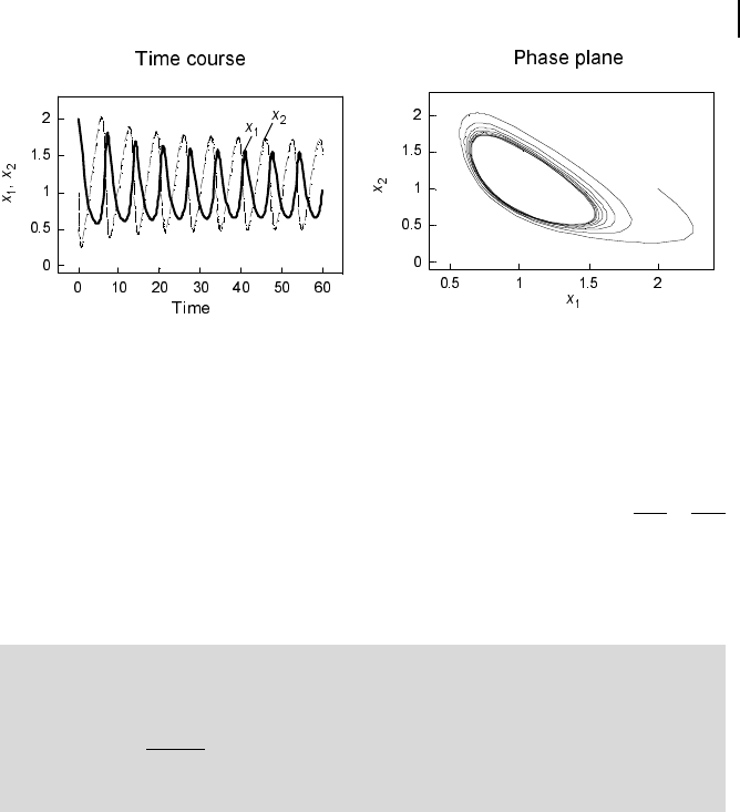
Example 3-11
The nonlinear system
_
x
1
= x
2
1
x
2
– x
1
,
_
x
2
= p – x
2
1
x
2
has a steady state at
x
1
= p,
x
2
=1/p.
Choosing, e.g., p = 0.98, this steady state is unstable since Trace A =1–p
2
>0.
Time course and phase plane behavior are shown in Fig. 3.3.
For two-dimensional systems there are two criteria for determining whether a
limit cycle exists. Consider the following system of differential equations:
74
3 Mathematics in a Nutshell
_
x
1
f
1
x
1
; x
2
(3-55)
_
x
2
f
2
x
1
; x
2
:
The negative criterion of Bendixson states: if the expression Trace =
if
1
ix
1
if
2
ix
2
does not change its sign in a certain region of the phase plane, then there is no
closed trajectory in this area. Hence, a necessary condition for the existence of a limit
cycle is a change in the sign of Trace.
Example 3-12
In Example 3-11 it holds that Trace =(2x
1
x
2
–1)+(–x
1
2
). Therefore, Trace =0 is
fulfilled at x
2
=
x
2
1
1
2 x
1
and Trace may assume positive or negative values for vary-
ing x
1
, x
2
and the necessary condition for the existence of a limit cycle is met.
The criteria of Poincaré-Bendixson states: if a trajectory in the phase plane re-
mains within a finite region without approaching a singular point (a steady state),
then this trajectory either is a limit cycle or it approaches a limit cycle. This criterion
gives a sufficient condition for the existence of a limit cycle. Nevertheless, the limit
cycle trajectory can be computed analytically only in very rare cases.
3.3
Difference Equations
Modeling with difference equations employs a discrete timescale, in contrast to the
continuous timescale in ODEs. For some processes, the value of the variable x at a
discrete time point t depends directly on the value of this variable at a former time
point. For example, the actual number of individuals in a population of birds in one
year can be related to the number of individuals last year.
75
3.3 Difference Equations
Fig. 3.3 Solution of the equation system in Example 3-11 represented
as time course and phase plane. Initial conditions: x
1
(0) = 2, x
2
(0) = 1.

A general (first-order) difference equation takes the form
x
i
f t; x
i1
for all t. (3-56)
We can solve such an equation by successive calculation: given x
0
, we have
x
1
f 1; x
0
x
2
f 2; x
1
f 2; f 1; x
0
: (3-57)
.
.
.
In particular, given any value x
0
, there exists a unique solution path x
1
, x
2
,…For
simple forms of the function f, we can also find general solutions.
Example 3-13
Consider the exponential growth of a bacterial population with a doubling of the
population size x
i
in each time interval. The recursive equation x
i
=2x
i–1
is
equivalent to the explicit equation x
i
= x
0
72
i
and also to the difference equation
x
i
– x
i–1
= Dx = x
i–1
.
The difference equation expresses the relation between values of a variable at dis-
crete time points. We are interested in the dynamics of the variable. For the gen-
eral case x
i
= rx
i–1
, it can be easily shown that x
i
= r
t
x
0
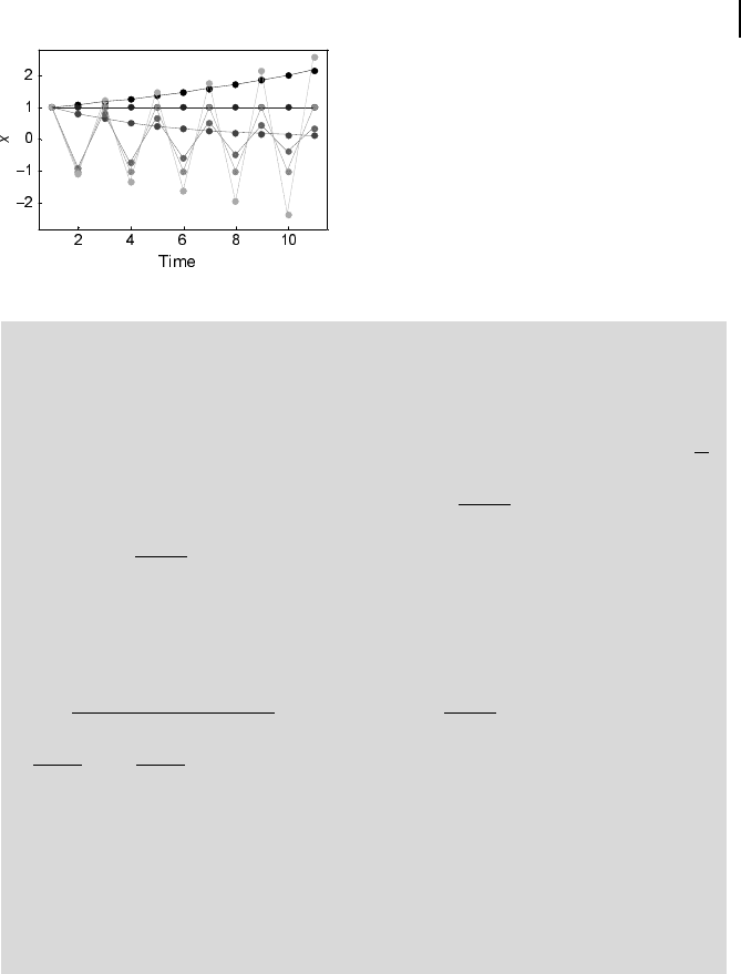
. This corresponds to the
law of exponential growth (Malthus’ law). The dynamic behavior depends on the
parameter r:
1<r: exponential growth
r =1: x remains constant, steady state
0<r < 1: exponential decay
–1 < r < 0: alternating decay
r = –1: periodic solution
r < –1: alternating increase
Example time courses are shown in Fig. 3.4.
A difference equation of the form
x
ik
fx
ik
; ...; x
i1
; x
i
(3-58)
is a k-th order difference equation. Like ODEs, difference equations may have sta-
tionary solutions that might be stable or unstable, which are defined as follows. The
value
x is a stationary solution or fix point of the difference equation (Eq. (3-58)) if
x = f (
x). A fix point is stable (or unstable), if there is a neighborhood N ={x:|x –
x|<e} such that every series that begins in N converges against
x (leaves N). The fol-
lowing sentence is practically applicable: the fix point is stable under the condition
that f is continuously differentiable if
df x
dx
x
< 1.
76
3 Mathematics in a Nutshell
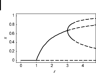
Example 3-14
The simplest form of the logistic equation, which plays a role in population dy-
namics, is x
n1
rx
n
1 x
n
, with fxrx 1 xwhere r is a positive valued
parameter. This difference equation has two fix points,
x
1
0 and
x
2
1
1
r
.
Stability analysis yields that fix point
x
1
is stable if
df x
dx
x
1
r < 1 and fix point
x
2
is stable if
df x
dx
x
2
2 r
jj
< 1; hence, 1 < r <3.
For r > 3 there are stable oscillations of period 2, i.e., successive generations alter-
nate between two values. Finding the steady states
x
1
and
x
2
is enabled by the
new function gx
ffx
. The equation g(x)=x has the two solutions
x
1;2
r 1
3 rr 1
p
2r
. They are stable if
dg x
dx
x
i
< 1 holds for i =1,2or
df x
dx
x
1
:
df x
dx
x
2
< 1, i.e., for 3 < r < 3.3. For r > 3.3, oscillations of
higher period occur, which can be treated in a manner analogous to oscillations of
period 2. For r > r
crit
chaos arises, i.e., albeit a deterministic description, the sys-
tem trajectories in fact cannot be reliably predicted and may differ remarkably for
close initial conditions. The points r =1,r = 3, and r = 3.3 are bifurcation points
since the number and stability of steady states change. A graphical representation
is given in Fig. 3.5.
3.4
Statistics
In this section we give an introduction to basic concepts of probability theory and
statistics. In practice, experimental measurements undergo some uncertainty (con-
centrations, RNA levels, etc.), and statistical concepts give us a framework to quan-
tify this uncertainty. Concepts of probability theory (Section 3.4.1) provide the neces-
sary mathematical models for computing the significance of the experimental out-
77
3.4 Statistics
Fig. 3.4 Temporal behavior of a difference equa-
tion describing exponential growth for various va-
lues of parameter r (r drops with the gray level).
come. The focus of elementary statistics (Section 3.4.2) is to describe the underlying
probabilistic parameters by functions on the experimental sample, the sample statis-
tics, and to provide tools for visualization of the data. Statistical test theory (Section
3.4.3) provides a framework for judging the significance of statements (hypotheses)
with respect to the data. Linear models (Section 3.4.4) are one of the most prominent
tools for analyzing complex experimental procedures.
3.4.1
Basic Concepts of Probability Theory
The quantification and characterization of uncertainty are formally described by the
concept of a probability space for a random experiment. A random experiment is an
experiment that consists of a set of possible outcomes with a quantification of the
possibility of such an outcome. For example, when a coin is tossed, one cannot deter-
ministically predict the outcome of “heads” or “tails” but rather assigns a probability
that either of the outcomes will occur. Intuitively, one will assign a probability of 0.5
if the coin is fair (i.e., both outcomes are equally likely). Random experiments are
described by a set of probabilistic axioms.
A probability space is a triplet (O, A, P) where O is a nonempty set, A is a s-alge-
bra of subsets of O, and P is a probability measure on A.As-algebra is a family of
subsets of O that (1) contains O itself, (2) contains for every element B B A the com-
plementary element B
c
B A, and (3) contains for every series of elements B
1
, B
2
,…,
B A their union, i.e.,
S
1
i1
B
i
B A. The pair (O, A) is called a measurable space. An
element of A is called an event. If O is discrete, i.e., it has at most countable many
elements, then a natural choice of A would be the power set of O, P(O), i.e., the set
of all subsets of O.
A probability measure P:A?[0,1] is a real-valued function that has the properties
P(B) 6 0 for all B B A and P(O)=1
and
P(
S
1
i1
B
i
)=
P
1
i1
P(B
i
) for all series of disjoint sets B
1
, B
2
,…,B A (s-additivity). (3-59)
78
3 Mathematics in a Nutshell
Fig. 3.5 Bifurcation diagram of the logistic equa-
tion. For increasing parameter r, the number of
steady-states increments are shown. At the points
r =1,r = 3, and r = 3.3, stability changes from
stable (solid lines) to unstable (dashed lines) oc-
cur. Only the constant solution and the solution of
periods 1 and 2 are shown.
Example 3-15: Urn models
Many practical problems can be described with urn models. Consider an urn con-
taining N balls of which K are red and N – K are black. The random experiment
consists of n draws from that urn. If the ball is replaced in the urn after each
draw we call the experiment drawing with replacement; otherwise, it is called
drawing without replacement. Here, O is the set of all n-dimensional binary se-
quences O ={(x
1
,…,x
n
); x
i
B {0,1}}, where a “1” means that a red ball was drawn
and a “0” means that a black ball was drawn. Since O is discrete, a suitable s-alge-
bra is the power set of O. Of practical interest is the calculation of the probability
of having exactly k red balls among the n balls drawn. This is given by
Pk
n
k
p
k
1 p
nk
, with p
K
N
, if we draw with replacement and
Pk
K
k
N K
n k
N
n
if we draw without replacement. Here for all numbers,
a 6 b 6 0 it is defined (binomial coefficients)
a
b
a!
a b!b!
: (3-60)
We can define the concept of conditional dependency. Let (O,A,P) be a probability
space and let B
1
, B
2
B A be two events. In general, there will be some dependency be-
tween the two events that influences the probability that both events will occur si-
multaneously. For example, consider B
1
as the event that a randomly picked person
has lung cancer and let B
2
be the event that the person is a smoker. If both events
were independent of each other, then the joint event B
1
\B
2
would be the product of
the probabilities, i.e., P(B
1
\B
2
)=P(B
1
)P (B
2
). This would mean that the probability
that a randomly picked person has lung cancer is independent of the fact that he is a
smoker. Otherwise, the probability of B
1
would be higher dependent on B
2
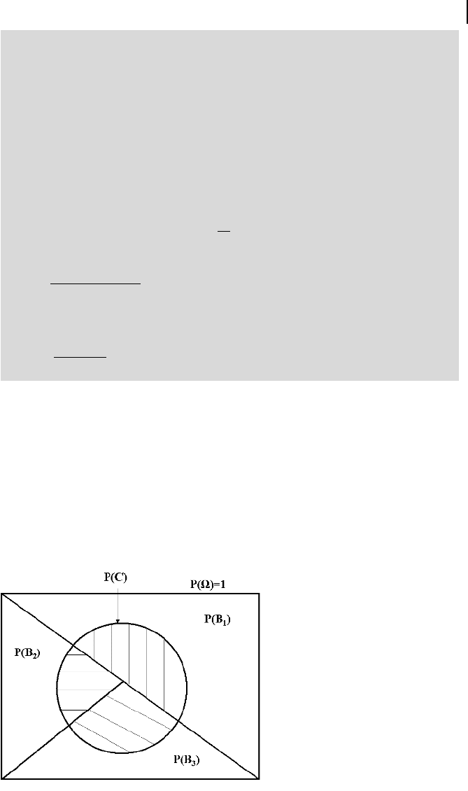
(Fig. 3.6).
79
3.4 Statistics
Fig. 3.6 Illustration of conditional
probabilities. Three events, B
1
, B
2
, B
3
,
build a partition of the probability space
O with a priori probabilities P(B
1
) = 0.5,
P(B
2
)=P(B
3
) = 0.25. Any event C de-
fines a conditional probability measure
with respect to C. Here, the a posteriori
probabilities given C are P(B
1
) = 0.5,
P(B
2
) = 0.17, P(B
3
) = 0.33, respectively.