Klipp E., Herwig R., Kowald A., Wierling C., Lehrach H. Systems Biology in Practice: Concepts, Implementation and Application
Подождите немного. Документ загружается.

PC
P
n
i1
x
i
x
:
y
i
y
:
P
n
i1
x
i
x
:
2
P
n
i1
y
i
y
:
2
s
: (3-87)
The Pearson correlation measures the linear relationship of both samples. It is
close to one if both samples have strong linear correlation, it is negative if the sam-
ples are anti-correlated, and it scatters around zero if there is no linear trend observa-
ble. Outliers can influence the Pearson correlation to a large extent. Therefore, ro-
90
3 Mathematics in a Nutshell
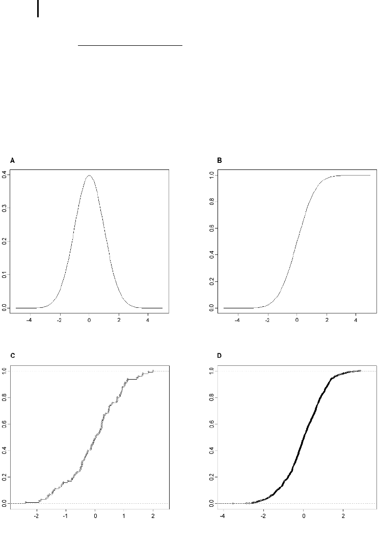
Fig. 3.8 Density function (A) and cumulative distribution function
(B) of a standard normal distribution with parameters m = 0 and
s = 1. Empirical distribution function of a random sample of 100 (C)
and 1000 (D) values drawn from a standard normal distribution.

bust statistics for sample correlation have been defined. We call r
i
x
=|{x
j
; x
j
^ x
i
}|
the rank of x
i
within the sample x
1
,…,x
n
. It denotes the number of sample values
smaller or equal to the i-th value. Note that the minimum, the maximum, and the
median of the sample have ranks, 1, n, and
n
2
, respectively, and that the ranks and
the ordered sample have the correspondence that x
i
= x
(r
i
x
)
. A more robust measure
of correlation than Pearson’s correlation coefficient is Spearman’s rank correlation
(SC):
SC
P
n
i1
r
x
i
r
x
:
r
y
i
r
y
:
P
n
i1
r
x
i
r
x
:
2
P
n
i1
r
y
i
r
y
:
2
s
: (3-88)
Here,
r
x
denotes the mean rank. SC is derived from PC by replacing the actual
sample values by their ranks within the respective sample. Another advantage of this
measure is the fact that SC can measure relationships other than linear ones. For ex-
ample, if the second sample is derived from the first by any monotonic function
(square root, logarithm), then the correlation is still high (Fig. 3.9). Measures of cor-
relation are extensively used in many algorithms of multivariate statistical analysis,
such as pairwise similarity measures for gene expression profiles (cf. Chapter 9).
3.4.3
Testing Statistical Hypotheses
Many practical applications imply statements such as “It is very likely that two sam-
ples are unequal” or “This fold change of gene expression is significant”. Consider
the following problems.
1. We observe the expression of a gene in replicated measurements of cells with a
chemical treatment and control cells. Can we quantify whether a certain fold
change in gene expression is significant?
2. We observe the expression of a gene in different individuals suffering from a cer-
tain disease and a control group. Is the variability in the two samples equal?
3. We measure gene expression of many genes. Does the signal distribution of these
genes resemble a specific distribution?
Statistical test theory provides a unique framework to tackle these questions and
to give numerical estimates for the significance of these differences.
3.4.3.1 Statistical Framework
Replicated measurements of the same object in a treatment and a control condition
typically yield two series of values, x
1
,…,x
n
and y
1
,…,y
m
. The biological problem of
judging differences from replicated measurements can be formulated as statistical
hypotheses: the null hypothesis, H
0
, and the alternative, H
1
.
91
3.4 Statistics
An important class of tests is the two-sample location test. Here, the null hypoth-
esis states that the difference between the two samples is zero, i.e., there is no differ-
ence, and the alternative states that there is a difference.
H
0
: m
x
m
y
versus H
1
: m
x
6 m
y
;
where m
x
, m
y
are the mean values of the respective samples.
92
3 Mathematics in a Nutshell
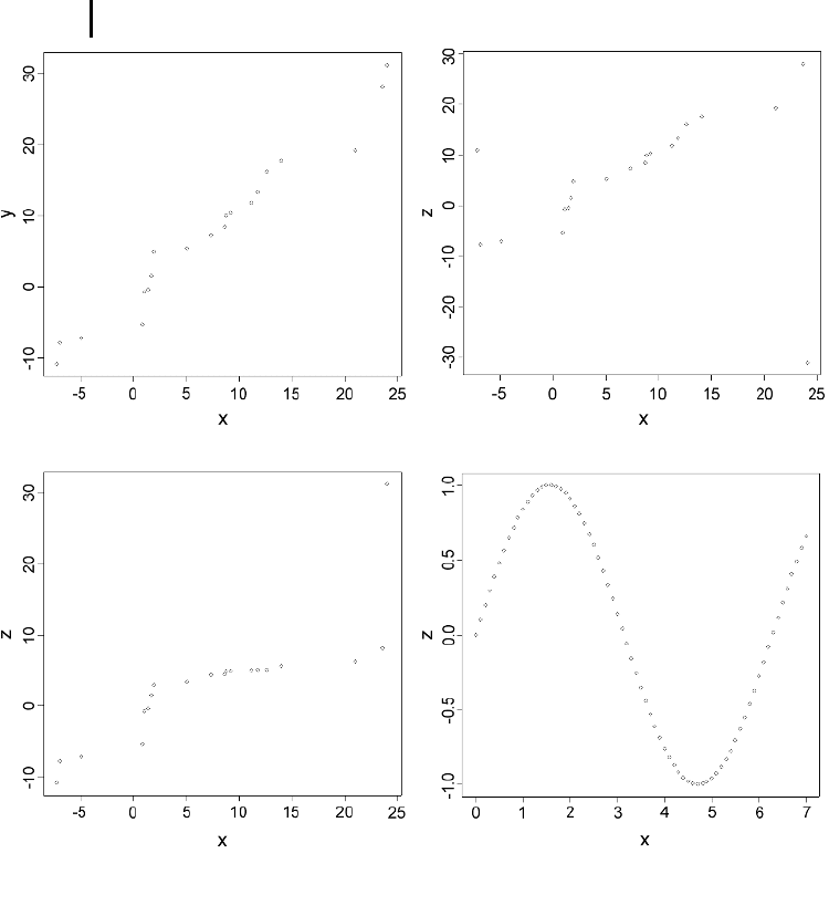
Fig. 3.9 Correlation plots and performance of correlation measures.
Top left: linear correlation of two random variables (PC = 0.98,
SP = 1.00); top right: presence of two outliers (PC = 0.27, SP = 0.60);
bottom left: nonlinear, monotonic correlation (PC = 0.83,
SP = 1.00); bottom right: nonlinear, non-monotonic correlation
(PC = –0.54, SP = –0.54).

A very simple argument would be to calculate the averages of the two series and
compare the ratios. However, this would not allow judging whether the ratio has any
significance. If we make some additional assumptions, we can describe the problem
using an appropriate probability distribution. We regard the two series as realiza-
tions of random variables x
1
,…,x
n
and y
1
,…,y
m
. Statistical tests typically have two
constraints: it is assumed that (1) repetitions are independent and (2) the random
variables are identically distributed within each sample. Test decisions are based
upon a reasonable test statistic, a real-valued function T, on both samples. For speci-
fic functions and using the distributional assumptions, it has been shown that they
follow a quantifiable probability law given the null hypothesis H
0
. Suppose that we
observe a value of the test statistic T (x
1
,…,x
n
, y
1
,…,y
m
)=
^
t.IfT could be described
with a probability law, we can then judge the significance of the observation by
prob(T more extreme than
^
t|H
0
). This probability is called a P-value. Thus, if one as-
signs a P-value of 0.05 to a certain observation, this means that under the distribu-
tional assumptions, the probability of observing an outcome more extreme than the
observed one is 0.05 given the null hypothesis. Observations with a small P-value ty-
pically give incidence that the null hypothesis should be rejected. This makes it pos-
sible to quantify statistically, using a probability distribution, whether the result is
significant. In practice, significance levels of 0.01, 0.05, and 0.1 are used as upper
bounds for significant results.
In such a test setup, two types of error occur: error of the first kind and error of
the second kind.
H
0
is true H
1
is true
Test does not reject H
0
No error (TN) Error of the second kind (FN)
Test rejects H
0
Error of the first kind (FP) No error (TP)
The error of the first kind is the false-positive (FP) rate of the test. Usually, this er-
ror can be controlled by the analysis by assuming a significance level of a and jud-
ging only those results where the probability is lower than a as significant. The error
of the second kind is the false-negative (FN) rate of the test. The power of a test (TP)
(given a significance level a) is defined as the probability of rejecting H
0
across the
parameter space that is under consideration. It should be low in the subset of the
parameter space that belongs to H
0
and high in the subset H
1
. The quantities
TP
TP FN
and
TN
FP TN
are called sensitivity and specificity, respectively. An optimal
test procedure would give a result of 1 to both quantities.
3.4.3.2 Two-sample Location Tests
Assume that both series are independently Gaussian distributed, N ( m
x
,s
2
) and
N( m
y
,s
2
) respectively, with equal variances. Thus we interpret each series value x
i
as
an outcome of independent random variables that are Gaussian distributed with the
respective parameters (y
i
likewise). We want to test the hypothesis of whether the
sample means are equal, i.e.,
93
3.4 Statistics

H
0
: m
x
m
y
versus H
1
: m
x
6 m
y
;
Under the above assumptions, the test statistic
T x
1
; :::; x
n
; y
1
; :::; y
m
x
:
y
:
n 1s
2
x
m 1s
2
y
n m 2
s
1
n
1
m
r
(3-89)
(compare Sections 3.4.2.1 and 3.4.2.2) and is distributed according to a t-distribution
with m + n – 2 degrees of freedom. Here, s
x
2
, s
y
2
denote the variances of the samples.
The test based on this assumption is called Student’s t-test.
For a calculated value of the t-statistic,
^
t, we can now judge the probability of hav-
ing an even more extreme value by calculating the probability P jTj > j
^
tj =
2 P T > j
^
tj =
R
1
^
t
f
T;p
zdz, where
f
T;p
z
G
p 1
2
G
p
2
G
1
2
p
p
1
z
2
p
p1=2
(3-90)
is the probability distribution of the respective t-distribution with p degrees of free-
dom. Here, Gz =
R
1
0
t
z1
e
t
dt is the gamma function.
For most practical applications, the assumptions of the Student’s t-test are too
strong, and data are not Gaussian distributed with equal variances. Furthermore,
since the statistic is based on the mean sample values, the test is not robust against
outliers. In cases where the underlying distribution is unknown and in order to de-
fine a more robust alternative, we introduce Wilcoxon’s rank sum test. Here, instead
of evaluating the signal values, only the ranks of the signals are taken into considera-
tion. Consider the combined series x
1
,…,x
n
, y
1
,…,y
m
. Under the null hypothesis
this series represents m + n independent identically distributed random variables.
The test statistic of the Wilcoxon test is
T
P
n
i1
R
x;y
i
; (3-91)
where R
i
x,y
is the rank of x
i
in the combined series. The minimum and maximum
values of T are
nn 1
2
and
m nm n 1
2
nn 1
2
, respectively. The ex-
pected value under the null hypothesis is E
H
0
T
n m n 1
2
and the variance is
Var
H
0
(T)=
mn m n 1
12
. Thus, under the null hypothesis, values for T will scatter
around the expectation, and unusually low or high values will indicate that the null
94
3 Mathematics in a Nutshell

hypothesis should be rejected. For small sample sizes, P-values of the Wilcoxon test
can be calculated exactly; for larger sample sizes, we have the following approxima-
tion:
P
T
n n m 1
2
mn m n 1
12
r
z
0
B
B
@
1
C
C
A
! F z for n; m !1: (3-92)
The P-values of the Wilcoxon test statistic can be approximated by the standard nor-
mal distribution. This approximation has been shown to be accurate for n + m>25.
In practice, some of the series values might be equal, e. g., because of the resolu-
tion of the measurements. Then, the Wilcoxon test statistic can be calculated using
ties. Ties can be calculated by the average rank of all values that are equal. Ties have
an effect on the variance of the statistic since this might be underestimated and
should be corrected in the normal approximation. The correction is calculated by re-
placing the original variance by
Var
H
0
;corr
TVar
H
0
T
mn
12 m nm n 1
X
r
i1
b
3
i
b
i
: (3-93)
Here, r is the number of different values in the combined series of values and b
i
is
the frequency.
Example 3-26
Expression of a specific gene was measured in cortex brain tissue from control
mice and Ts65Dn mice – a mouse model for Down syndrome (Kahlem et al.
2004). Repeated array hybridization experiments yield the following series of
measurements for control mice
2434 2289 5599 2518 1123 1768 2304 2509 14820 2489 1349 1494
and for trisomic mice
3107 3365 4704 3667 2414 4268 3600 3084 3997 3673 2281 3166.
Due to two outlier values in the control series (5599 and 14820) the trisomic ver-
sus control ratio is close to one, 1.02, and the P-value of Student’s t-test is not sig-
nificant, p = 9.63e – 01. For the Wilcoxon statistic, we get T=
P
n
i1
R
x;y
i
= 14 + 16 +
22 + 18 + 8 + 21 + 17 + 13 + 20 + 19 + 5 + 15 = 188, E
H
0
(T) = 150,Var
H
0
(T) = 300,
and for the Z-score we have z=
38
300
p
~ 2.19, which indicates that the result is sig-
nificant. The exact P-value of the Wilcoxon test is p = 2.84e – 02.
95
3.4 Statistics

3.4.4
Linear Models
The general linear model has the form y = Xb + e, with the assumptions E(e)=0 and
Cov(e)=r
2
I. Here y is an n-dimensional vector of observations, b is a p-dimensional
vector of unknown parameters, X is an nxp dimensional matrix of known constants
(the design matrix), and e is a vector of random errors. Since the errors are random,
y is a random vector as well. Thus, the observations are separated into a determinis-
tic part and a random part. The rationale behind linear models is that the determi-
nistic part of the experimental observations is a linear function of the design matrix
and the unknown parameter vector. Note that linearity is required in the parameters,
not in the design matrix. For example, problems such as x
ij
= x
j
i
for i = 1, …, n and
j = 0, …, p – 1 are also linear models. Here, for each coordinate i we have the equa-
tion y
i
= b
0
+
P
p1
j1
b
j
x
i
j
+ e
i
and the model is called the polynomial regression model.
The goal of linear models is testing of complex statistical hypotheses and para-
meter estimation (cf. Chapter 9). In the following sections we introduce two classes
of linear models: analysis of variance (ANOVA) and regression.
3.4.4.1 ANOVA
In Section 3.4.3.2 we introduced a particular test problem, the two-sample location
test. The purpose of this test is to judge whether or not two samples are drawn from
the same population by comparison of the centers of these samples. The null hy-
pothesis was H
0
:m
1
= m
2
and the alternative hypothesis was H
1
:m
1
= m
2
, where m
i
is
the mean of the i-th sample. A generalization of the null hypothesis is targeted in
this section. Assume n different samples where each sample measures the same in-
teresting factor. Within each sample, i, the factor is measured n
i
times. This results
in a table of the following form
x
11
x
21
::: x
n1
::: :: ::: :::
x
1n
1
x
2n
2
::: x
nn
n
Here, the columns correspond to the different individual samples, and the rows
correspond to the individual repetitions within each sample (the number of rows
within each sample can vary!). The interesting question now is whether there is any
difference in the sample means or, alternatively, whether the samples represent the
same population. We thus test the null hypothesis H
0
:m
1
= m
2
=…=m
n
against the
alternative H
1
:m
i
= m
j
for at least one pair, i = j. This question is targeted by the so-
called one-way ANOVA. As in the case of Student’s t-test, additional assumptions on
the data samples are necessary:
1. The n samples are drawn independently from each other representing populations
with mean values m
1
, m
2
,…,m
n
.
2. All population variances have the same variance s
2
(homoscedasticity).
3. All populations are Gaussian distributed, N(m
i
, s
2
).
96
3 Mathematics in a Nutshell
Although, the one-way ANOVA is based on the analysis of variance, it is essen-
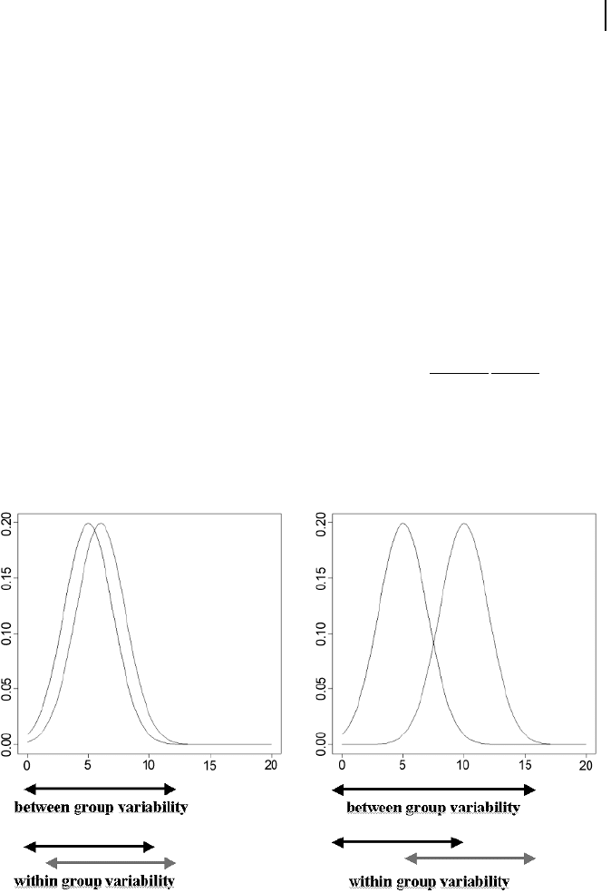
tially a test for location. This is exemplified in Fig. 3.10. The idea of ANOVA is the
comparison of between- and within-group variability. If the variance between the
groups is not different from the variance within the groups, we cannot reject the
null hypotheses (Fig. 3.10, left). If the variances differ, we would reject the null hy-
pothesis and conclude that the means are different (Fig. 3.10, right).
The calculation of the one-way ANOVA is based on the partition of the sample var-
iance
P
n
i1
P
n
i
j1
x
ij
x
::
2
into two parts that account for the between- and within-group
variability, i.e.,
SS
total
P
n
i1
P
n
i
j1
x
ij
x
::
2
P
n
i1
P
n
i
j1
x
i:
x
::
2
P
n
i1
P
n
i
j1
x
ij
x
i:
2
SS
between
SS
within
:
(3-94)
It can be shown that under H
0
the test statistic T
SS
between
SS
within
M n
n 1
, where
M
P
n
i1
n
i
, is distributed according to an F distribution with degrees of freedom
n
1
= n – 1 and n
2
= M – n, respectively. The multiplicative constant accounts for the
degrees of freedom of the two terms. Thus, we can quantify experimental outcomes
97
3.4 Statistics
Fig. 3.10 ANOVA test for differential expression. Left: two normal
distributions with means m
1
=5,m
2
= 6 and equal variances. The
variability between the groups is comparable with the variability
within the groups. Right: two normal distributions with means
m
1
=5,m
2
= 10 and equal variances. The variability between the
groups is higher than the variability within the groups.

according to this distribution. If m
i
are not equal, SS
between
will be high compared to
SS
within
, and, conversely, if all m
i
are equal, then the two factors will be similar and T
will be small.
3.4.4.2 Multiple Linear Regression
Let y be an n-dimensional observation vector and let x
1
,…,x
p–1
be independent n-di-
mensional variables. We assume that the number of observations is greater than the
number of variables, i.e., n > p. The standard model here is
y Xb e (3-95)
or, in matrix notation,
y
1
.
.
.
y
n
0
B
@
1
C
A
1 x
11
x
p1;1
.
.
.
.
.
.
.
.
.
.
.
.
1 x
1n
x
p1;n
0
B
B
@
1
C
C
A
b
0
.
.
.
b
p1
0
B
@
1
C
A
e
1
.
.
.
e
n
0
B
@
1
C
A
where E (e) = 0 and Va r (e)=r
2
I
n
. In our model we are interested in an optimal es-
timator for the unknown parameter vector b. The least-squares method defines
this optimization as a vector
^
b that minimizes the Euclidean norm of the resi-
duals, i. e.,
^
b 2 arg min b; y Xb
2
no
Using partial derivatives, we can transform this problem into a linear equation (cf.
Section 3.1.1) system by
X
T
Xb X
T
y (3-96)
and get the solution
^
b X
T
X
1
X
T
y : (3-97)
The solution is called the least-squares estimator for b. The least-squares estimator
is unbiased, i.e., E(
^
b = b and the covariance matrix R
^
b
of
^
b is equal to R
^
b
=
r
2
(X
T
X)
–1
. Through the estimator for b, we have an immediate estimator for the er-
ror vector e using the residuals
^
e y X
^
b y X X
T
X
1
X
T
y y Py : (3-98)
Geometrically, P is the projection of y in the p-dimensional subspace of <
n
that is
spanned by the column vectors of X.
98
3 Mathematics in a Nutshell

An unbiased estimator for the unknown standard deviation s
2
is given by
^
s
2
y X
^
b
2
n p
: (3-99)
Thus, E
^
s
2
s
2
.
Example 3-27: Simple linear regression
An important application is the simple linear regression of two samples x
1
,…,x
n
and y
1
,…,y
n
. Here Eq. (3-95) reduces to
y
1
.
.
.
y
n
0
B
@
1
C
A
1 x
1
.
.
.
.
.
.
1 x
n
0
B
@
1
C
A
b
0
b
1
e
1
.
.
.
e
n
0
B
@
1
C
A
and
the parameters of interest are b
0
, b
1
, the intercept and the slope of the regression
line. Minimizing the Euclidean norm of the residuals computes the line that
minimizes the vertical distances of all points to the regression line. Solving ac-
cording to Eq. (3-97) gives
X
T
X
n
P
n
i1
x
i
P
n
i1
x
i
P
n
i1
x
2
i
0
B
B
@
1
C
C
A
and X
T
y
P
n
i1
y
i
P
n
i1
x
i
y
i
0
B
B
@
1
C
C
A
, and thus we have
^
b
1
n
P
n
i1
x
2
i
P
n
i1
x
i
2
P
n
i1
x
2
i
P
n
i1
x
i
P
n
i1
x
i
n
0
B
B
@
1
C
C
A
P
n
i1
y
i
P
n
i1
x
i
y
i
0
B
B
@
1
C
C
A
1
n
P
n
i1
x
2
i
P
n
i1
x
i
2
P
n
i1
x
2
i
P
n
i1
y
i
P
n
i1
x
i
P
n
i1
x
i
y
n
P
n
i1
x
i
y
i
P
n
i1
x
i
P
n
i1
y
i
0
B
B
@
1
C
C
A
The slope of the regression line is the correlation of the samples divided by the
variance of the variables. It is called the empirical regression coefficient.
3.5
Graph and Network Theory
Many kinds of data arising in systems biology applications can be represented as
graphs (metabolic pathways, signaling pathways, or gene regulatory networks).
Other examples are taxonomies, e.g., of enzymes or organisms; protein interaction
networks; DNA, RNA, or protein sequences; chemical structure graphs; or gene
co-expression. In this section we give a brief overview of the formalization of graph
problems (Section 3.5.1) and introduce specifically the framework of gene regula-
99
3.5 Graph and Network Theory