Krantz W.B. Scaling Analysis in Modeling Transport and Reaction Processes: A Systematic Approach to Model Building and the Art of Approximation

Подождите немного. Документ загружается.

EXAMPLE PROBLEMS 83

∗

∂

∂r

∗

) +

∂u

∗

∂z

∗

= 0 (3.E.4-19)

∗

= 0,u

∗

= 0,u

∗

ωr

θs

∗

at z

∗

= 0 (3.E.4-20)

∗

=−

∞

∗

= 0,u

∗

= 0,P

∗

∞

− P

as z

∗

→∞ (3.E.4-21)

∗

= 0,u

∗

= 0atr

∗

= 0 (3.E.4-22)

We now apply step 7 to achieve

◦

(1) scaling. Since we seek to describe the ﬂow

at any arbitrary position along the disk, we set r

= R, the local radial coordinate;

that is, we are considering a local scaling analysis. The appropriate dimension-

less groups in equations (3.E.4-20) and (3.E.4-21) suggest the following scale and

reference factors:

θs

ωr

θs

ωR

= 1 ⇒ u

θs

= ωR;

∞

− P

= 0 ⇒ P

= P

∞

(3.E.4-23)

Since this is a developing ﬂow, the continuity equation given by (3.E.4-19) implies

that

= 1 ⇒ u

(3.E.4-24)

The scale for u

is obtained from equation (3.E.4-16) since the inertia and viscous

terms must balance:

ρu

θs

μu

ρRω

μu

= 1 ⇒ u

ρRω

⇒ u

ρω

(3.E.4-25)

Similarly, the inertia and viscous terms in equation (3.E.4-18) must balance, which

provides the axial length scale:

ρu

= 1 ⇒ z

≡ δ



ρω



(3.E.4-26)

where ν is the kinematic viscosity. The axial length scale z

has been identiﬁed with

the momentum boundary-layer thickness δ

, the region of inﬂuence within which

the ﬂuid is affected by the rotating disk. Note that in contrast to most boundary-

layer problems in ﬂuid dynamics, δ

is constant over the entire surface of the

rotating disk. Finally, the pressure scale is also obtained from equation (3.E.4-18):

μu

ρω

1/2

3/2

= 1 ⇒ P

ρω

1/2

3/2

(3.E.4-27)

84 APPLICATIONS IN FLUID DYNAMICS

Substitution of the scale and reference factors then yields the following set of

dimensionless describing equations:

∗

∂u

∗

∂r

∗

−

∗2

∗

+ u

∗

∂u

∗

∂z

∗

∂

∗

∂z

∗2

(3.E.4-28)

∗

∂u

∗

∂r

∗

+ u

∗

∂u

∗

∂z

∗

∂

∗

∂z

∗2

(3.E.4-29)

∗

=−

∗

∗2

(3.E.4-30)

∗

∂

∂r

∗

) +

∂u

∗

∂z

∗

= 0 (3.E.4-31)

∗

= 0,u

∗

= 0,u

∗

= r

∗

at z

∗

= 0 (3.E.4-32)

∗

=−

∞

√

ων

∗

=, 0,u

∗

= 0,P

∗

= 0asz

∗

→∞ (3.E.4-33)

∗

= 0,u

∗

= 0atr

∗

= 0 (3.E.4-34)

Equations (3.E.4-28) through (3.E.4-34) have been solved via a series-expansion

method (see footnote 17). The resulting series can be truncated at the ﬁrst term if

 1 corresponding to a very thin momentum boundary layer. The resulting solu-

tion indicates that δ

= 3.6

√

ν/ω and U

∞

= 0.88447

√

νω. These agree to within

a constant of

◦

(1) with the estimates obtained for δ

given by equation (3.E.4-26)

and for U

∞

obtained by setting the dimensionless group in equation (3.E.4-33)

equal to 1. Note that scaling has provided reliable estimates of both the momentum

boundary-layer thickness δ

and the far-ﬁeld axial velocity U

∞

without the need

to actually solve the describing equations.

To assume that the rotating disk is effectively in an unbounded ﬂuid, it is nec-

essary for the boundary layer to be very thin; that is, the following criterion must

be satisﬁed (step 8):



ωH

 1or



ωH

◦

(0.01) (3.E.4-35)

where H denotes the distance of the rotating disk from the nearest parallel bound-

ary. This condition will be satisﬁed when the kinematic viscosity is low, the angular

rotation rate is high, or the boundary is far removed from the rotating disk.

3.E.5 Entry Region Flow Between Parallel Plates

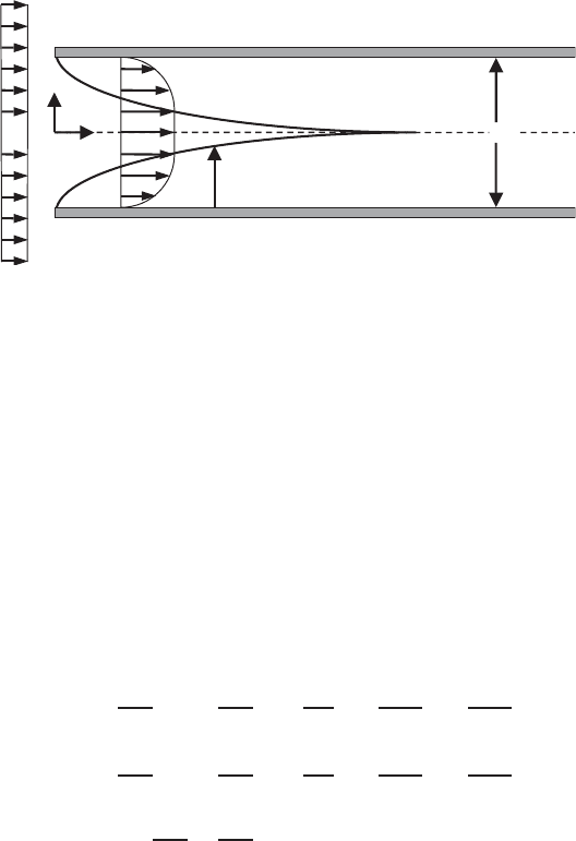
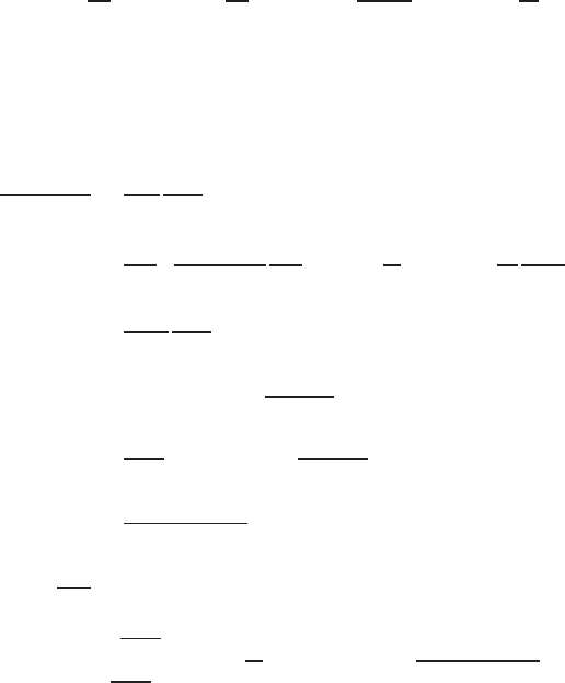
Figure 3.E.5-1 shows a schematic of pressure-driven steady-state laminar entry-

region ﬂow of an incompressible Newtonian ﬂuid with constant physical properties

between two parallel ﬂat plates spaced a distance 2H apart. The constant ﬂow

velocity at the entrance is U

. This is assumed to be a high Reynolds number

laminar ﬂow for which the inertia or convection terms cannot be ignored in the entry

EXAMPLE PROBLEMS 85

(x)

Figure 3.E.5-1 High Reynolds number steady-state pressure-driven entry region ﬂow of

an incompressible Newtonian ﬂuid with constant physical properties between two parallel

ﬂat plates spaced a distance 2H apart.

region. We will use scaling to estimate the entry length required to achieve fully

developed laminar ﬂow. Note that this ﬂow differs somewhat from the boundary-

layer ﬂow considered in Section 3.4 in that this is a conﬁned boundary-layer ﬂow.

Hence, owing to the deceleration of the ﬂow within the boundary layer at the walls,

the uniform or plug ﬂow in the center must accelerate. Moreover, in contrast to the

boundary-layer ﬂow considered in Section 3.4 that was caused by the velocity of

the ﬂow external to the boundary layer, the ﬂow in the present example is caused

by an applied pressure gradient.

The describing equations are obtained by simplifying equations (C.1-1),

(D.1-10), and (D.1-11) in the Appendices appropriately (step 1):

ρu

∂u

∂x

+ ρu

∂u

∂y

=−

∂P

∂x

+ μ

∂

∂x

+ μ

∂

∂y

(3.E.5-1)

ρu

∂u

∂x

+ ρu

∂u

∂y

=−

∂P

∂y

+ μ

∂

∂x

+ μ

∂

∂y

(3.E.5-2)

∂u

∂x

∂u

∂y

= 0 (3.E.5-3)

= U

= 0,P= P

at x = 0 (3.E.5-4)

= f

(y), u

= f

(y) at x = L (3.E.5-5)

= 0,u

= 0aty =±H (3.E.5-6)

= f

(x), u

= f

(x) at y =±(H − δ

) (3.E.5-7)

where f

(y) and f

(y) are unspeciﬁed functions of y and f

(x) and f

(x) are

unspeciﬁed functions of x that in principle would have to be known in order to

integrate the set of differential equations above. Note that we have introduced a

region of inﬂuence δ

(x) within which the effect of the viscous shear induced by

the presence of each wall is conﬁned. The rationale for introducing this region of

86 APPLICATIONS IN FLUID DYNAMICS

inﬂuence or hydrodynamic boundary-layer thickness was discussed in Section 3.4.

The set of equations above also introduces the pressure P

that would have to be

speciﬁed at the entry region in order to integrate the system of equations above.

Introduce the following scale factors, reference factors, and dimensionless vari-

ables (steps 2, 3, and 4):

∗

≡

; u

∗

≡

; P

∗

≡

; x

∗

≡

; y

∗

≡

y −y

(3.E.5-8)

We have introduced a reference factor y

in the deﬁnition of y

∗

to force this dimen-

sionless variable to zero at the wall. Note that the symmetry of this problem permits

considering only the region −H ≤ y ≤ 0. Substituting these dimensionless variables

into equations (3.E.5-1) through (3.E.5-7) and dividing through by the dimensional

coefﬁcient of one of the principal terms in each equation then yields the following

equations that describe the ﬂow in the region −H ≤ y ≤ 0 (steps 5 and 6):

∗

∂u

∗

∂x

∗

∂u

∗

∂y

∗

=−

ρu

∂P

∗

∂x

∗

ρu

∂

∗

∂x

∗2

μx

ρu

∂

∗

∂y

∗2

(3.E.5-9)

∗

∂u

∗

∂x

∗

∂u

∗

∂y

∗

=−

ρu

∂P

∗

∂y

∗

ρu

∂

∗

∂x

∗2

μx

ρu

∂

∗

∂y

∗2

(3.E.5-10)

∂u

∗

∂x

∗

∂u

∗

∂y

∗

= 0 (3.E.5-11)

∗

= 0,P

∗

at x

∗

= 0 (3.E.5-12)

∗

= f

∗

), u

∗

= f

∗

) at x

∗

(3.E.5-13)

∗

= 0,u

∗

= 0aty

∗

=−

H − y

(3.E.5-14)

∗

= f

∗

), u

∗

= f

∗

) at y

∗

=−

H − δ

− y

(3.E.5-15)

We now apply step 7 to bound the variables to be

◦

(1). We can bound y

∗

to be

between 0 and 1 by setting the dimensionless groups in equations (3.E.5-14) and

(3.E.5-15) equal to zero and 1, respectively, to obtain y

= H and y

= δ

.The

axial length scale can be bounded to be between 0 and 1 by setting the dimen-

sionless group in equation (3.E.5-13) equal to 1, thereby obtaining x

= L.The

axial velocity can be bounded to be between 0 and 1 by setting the dimensionless

group in equation (3.E.5-12) equal to 1, thereby obtaining u

= U

. Since this is a

developing ﬂow, both terms in the dimensionless continuity equation should be of

the same order; hence, we require that the dimensionless group in equation (3.E.5-

11) be equal to 1, thereby obtaining u

= U

/L. Since this is a pressure-driven

EXAMPLE PROBLEMS 87

high Reynolds number ﬂow, the dimensionless pressure term should be of the same

order as the inertia terms; hence, we require that dimensionless group multiplying

the pressure term in equation (3.E.5-9) be equal to 1, thereby obtaining P

= ρU

The resulting scaled dimensionless describing equations are given by

∗

∂u

∗

∂x

∗

+ u

∗

∂u

∗

∂y

∗

=−

∂P

∗

∂x

∗

∂

∗

∂x

∗2

∂

∗

∂y

∗2

(3.E.5-16)

∗

∂u

∗

∂x

∗

+ u

∗

∂u

∗

∂y

∗

=−

∂P

∗

∂y

∗

∂

∗

∂x

∗2

∂

∗

∂y

∗2

(3.E.5-17)

∂u

∗

∂x

∗

∂u

∗

∂y

∗

= 0 (3.E.5-18)

∗

= 1,u

∗

= 0,P

∗

ρU

at x

∗

= 0 (3.E.5-19)

∗

= f

∗

), u

∗

= f

∗

) at x

∗

= 1 (3.E.5-20)

∗

= 0,u

∗

= 0aty

∗

= 0 (3.E.5-21)

∗

= f

∗

), u

∗

= f

∗

) at y

∗

= 1 (3.E.5-22)

where Re ≡ δ

ρU

/μ is the Reynolds number. The principal viscous term in

equation (3.E.5-16) must be of the same size as the pressure and inertia terms

within the region of inﬂuence (hydrodynamic boundary layer) if we are to sat-

isfy the boundary conditions given by equations (3.E.5-21) and (3.E.5-22). Hence,

we require that the dimensionless group multiplying the principal viscous term in

equation (3.E.5-16) be equal to 1, which provides an estimate of the boundary-layer

thickness δ

∗

= 1 ⇒ δ



μL

ρU

(3.E.5-23)

When the boundary layer thickness δ

= H , the ﬂow is fully developed. Hence,

we can use equation (3.E.5-23) evaluated at δ

= H to obtain an estimate of the

entrance length L

∼

ρU

(3.E.5-24)

This agrees to within a multiplicative constant of order 1 with the entrance length

required to achieve fully developed ﬂow obtained from solving the boundary-layer

equations that yields

= 0.16

ρU

(3.E.5-25)

See H. Schlichting, Boundary Layer Theory, 4th ed., McGraw-Hill, New York, 1980, p. 168.

88 APPLICATIONS IN FLUID DYNAMICS

Whereas for this well-studied ﬂow, an equation is available to predict the entrance

length that obviates the need to use scaling analysis, the latter provides an invaluable

tool for estimating the entry region for ﬂows for which no such results are available.

Equations (3.E.5-16) through (3.E.5-23) can be greatly simpliﬁed if δ

◦

(0.01) (step 8). This permits ignoring the axial diffusion of vorticity term in

equation (3.E.5-16), thereby obviating the need to satisfy any downstream boundary

condition. Moreover, in view of equation (3.E.5-17), this condition implies that the

dimensionless derivative ∂P

∗

/∂y

∗

is very small. Note that we have not scaled the

dimensionless derivative ∂P

∗

/∂y

∗

in equation (3.E.5-17) to be

◦

(1) since there is

no reason for this derivative to scale as P

. However, since we have scaled

∗

∂u

∗

/∂x

∗

to be of order

◦

(1), equation (3.E.5-17) implies that ∂P

∗

/∂y

∗

is of

◦

(δ

) and hence that it is very small. This decouples the solution of equation

(3.E.5-16) from equation (3.E.5-17) and implies that the dimensionless describing

equations for the entry-region ﬂow problem can be reduced to

∗

∂u

∗

∂x

∗

+ u

∗

∂u

∗

∂y

∗

=−

∗

∂

∗

∂y

∗2

(3.E.5-26)

∂u

∗

∂x

∗

∂u

∗

∂y

∗

= 0 (3.E.5-27)

∗

= 1,u

∗

= 0,P

∗

ρU

at x

∗

= 0 (3.E.5-28)

∗

= 0,u

∗

= 0aty

∗

= 0 (3.E.5-29)

∗

= f

∗

) at y

∗

= 1 (3.E.5-30)

To solve equations (3.E.5-26) through (3.E.5-30), it is necessary to know the unspe-

ciﬁed function f

∗

) in equation (3.E.5-30). This is obtained by solving the ideal

ﬂow (inviscid) ﬂow equations

outside the boundary-layer region for which vis-

cous effects can be ignored, due to the high Reynolds number. In doing this, one

carries out integral mass and momentum balances that account for the acceler-

ation of the ﬂow due to the thinning of the inviscid core region that is caused

by the growing boundary layer at each wall. These equations can then be solved

analytically to determine the unspeciﬁed function f

∗

) in equation (3.E.5-30).

Equations (3.E.5-26) and (3.E.5-27) can then be solved numerically. The resulting

solution will yield the entrance length given by equation (3.E.5-25).

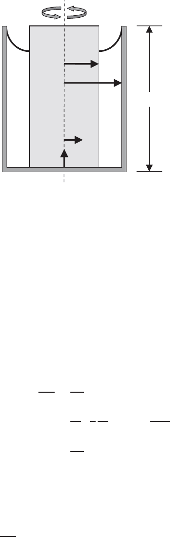
3.E.6 Rotating Flow in an Annulus with End Effects

Consider the steady-state ﬂow of an incompressible Newtonian liquid with con-

stant physical properties in the annular region between two concentric cylinders

of length L, shown in Figure 3.E.6-1. The inner cylinder has radius R

and is

The ideal or inviscid ﬂow equations correspond to an inﬁnite Reynolds number, which implies no

viscous effects whatsoever; in the case of hydrodynamic boundary-layer ﬂows, the ﬂow region outside

the boundary layer is described by the ideal ﬂow equations.

EXAMPLE PROBLEMS 89

Figure 3.E.6-1 Steady-state incompressible laminar ﬂow of a Newtonian liquid with con-

stant physical properties in the annular region between a stationary inner and a rotating outer

cylinder.

stationary. The outer cylinder has radius R

and rotates at a constant angular veloc-

ity ω (radians per second). The ﬂow is caused primarily by the rotation of the outer

cylinder. However, the bottom of the outer cylinder is also rotating and dragging

the adjacent liquid with it, causing an end effect. We neglect any effect of the

small gap between the bottom of the stationary inner cylinder and the rotating

outer cylinder. We use scaling analysis to derive criteria for ignoring the end effect

on the primary rotational ﬂow in the annulus.

The describing equations for this ﬂow are obtained by appropriately simplifying

the equations of motion in cylindrical coordinates given by equations (D.2-10)

through (D.2-12) in the Appendices (step 1):

ρu

∂P

∂r

(3.E.6-1)

0 =

∂

∂r



∂

∂r

(ru

)



∂

∂z

(3.E.6-2)

0 =

∂P

∂z

+ ρg (3.E.6-3)

= 0atr = R

(3.E.6-4)

= ωR

at r = R

(3.E.6-5)

= ωr at z = 0 (3.E.6-6)

∂u

∂z

= 0atz = f

(r) (3.E.6-7)

90 APPLICATIONS IN FLUID DYNAMICS

The boundary condition given by equation (3.E.6-7) allows for the fact that the

rotation causes a centrifugal pressure force that increases with the radius. At any

point in the liquid the centrifugal pressure has to be balanced by the hydrostatic

pressure. Hence, the liquid depth will increase with increasing radius. The location

of this interface can be determined from the solution to the pressure proﬁle. The

function f

(r) must satisfy the integral conservation of mass for an incompressible

liquid given by



2πrf

(r) dr = π(R

− R

(3.E.6-8)

where L

is the liquid depth in the absence of any rotation.

Introduce the following scale factors, reference factor, and dimensionless vari-

ables (steps 2, 3, and 4):

∗

≡

; P

∗

≡

; r

∗

≡

r − r

; z

∗

≡

(3.E.6-9)

We have introduced a reference factor for the dimensionless radial coordinate since

r is not naturally referenced to zero within the region where ﬂow is occurring.

Substitute these dimensionless variables into the describing equations and divide

through by the dimensional coefﬁcient of a term that must be retained (steps 5 and 6):

∗2

∗

+ r

ρu

∂P

∗

∂r

∗

(3.E.6-10)

0 =

∂

∂r

∗



∗

+ r

∂

∂r

∗



∗



∗



∂

∗

∂z

∗2

(3.E.6-11)

0 =

ρgz

∂P

∗

∂z

∗

+ 1 (3.E.6-12)

∗

= 0atr

∗

− r

(3.E.6-13)

∗

ωR

at r

∗

− r

(3.E.6-14)

∗

ωr

∗

+ r

at z

∗

= 0 (3.E.6-15)

∂u

∗

∂z

∗

= 0atz

∗

= f

∗

) (3.E.6-16)



−r



∗



∗



∗



∗



− R



(3.E.6-17)

We now apply step 7 to bound the variables to be

◦

(1). We can bound r

∗

be between zero and 1 by setting the dimensionless group in equation (3.E.6-13)

equal to zero and that in equation (3.E.6-14) equal to 1, thereby obtaining r

= R

EXAMPLE PROBLEMS 91

and r

= R

− R

. Our dimensionless axial coordinate can be bounded between

zero and 1 by setting the dimensionless group L

that appears in equation

(3.E.6-17) equal to 1, thereby obtaining z

= L

. Our velocity scale is obtained

from the dimensionless group in equation (3.E.6-14) to obtain u

= ωR

. Finally,

our pressure scale is obtained from the dimensionless group in equation (3.E.6-10)

to obtain P

= ρω

. When these scale and reference factors are substituted in

equations (3.E.6-10) through (3.E.6-17), we obtain the following set of dimension-

less describing equations:

∗2

∗

+ R

/(R

− R

)

∂P

∗

∂r

∗

(3.E.6-18)

0 =

∂

∂r

∗



∗

+ R

/(R

− R

)

∂

∂r

∗



∗

− R



∗



− R

)

∂

∗

∂z

∗2

(3.E.6-19)

0 =

∂P

∗

∂z

∗

+ 1 (3.E.6-20)

∗

= 0atr

∗

= 0 (3.E.6-21)

∗

= 1atr

∗

= 1 (3.E.6-22)

∗

− R



∗

− R



at z

∗

= 0 (3.E.6-23)

∂u

∗

∂z

∗

= 0atz

∗

= f

∗

) (3.E.6-24)





∗

− R



∗



∗



∗

+ R

− R

(3.E.6-25)

We see that if the dimensionless group (R

− R

)

◦

(0.01) the end effect

can be ignored in equation (3.E.6-19) (step 8). The resulting simpliﬁed set of

describing equations can be solved analytically.

A further simpliﬁcation is possi-

ble if the group (R

− R

)/R

◦

(0.01), in which case the describing equations

reduce to

0 =

∂P

∗

∂r

∗

(3.E.6-26)

0 =

∗

∗2

(3.E.6-27)

0 =

∂P

∗

∂z

∗

+ 1 (3.E.6-28)

This simpliﬁed set of describing equations has been solved in Bird et al., Transport Phenomena, 2nd

ed., pp. 93–95; however, no attempt is made to justify when these simpliﬁed equations are applicable.

92 APPLICATIONS IN FLUID DYNAMICS

∗

= 0atr

∗

= 0 (3.E.6-29)

∗

= 1atr

∗

= 1 (3.E.6-30)



∗



∗



∗

= 1 (3.E.6-31)

This simpliﬁed set of describing equations also admits an analytical solution.

The integral mass-balance condition is retained in the form given by equation

(3.E.6-31), which permits obtaining the liquid depth proﬁle in the annular region.

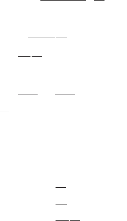
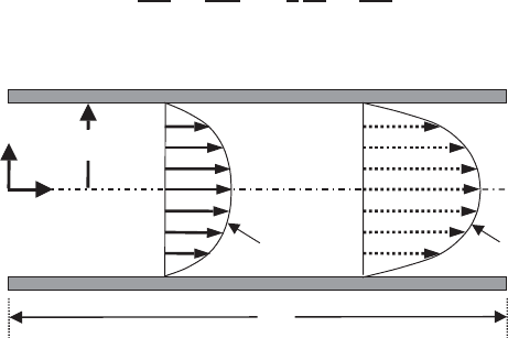
3.E.7 Impulsively Initiated Pressure-Driven Laminar Tube Flow

Consider an incompressible Newtonian liquid with constant physical properties

contained in a semi-inﬁnitely long cylindrical tube having radius R. Initially, the

liquid in the tube is at rest. At time t = 0, a constant pressure drop P ≡ P

− P

is applied across some length L of the tube to initiate continuous ﬂow, as shown

in Figure 3.E.7-1. We will ignore any entrance effects, in which case this is an

interesting example of an unsteady-state fully developed ﬂow. Figure 3.E.7-1 shows

the axial velocity proﬁles at times t

and t

,wheret

. If the entrance effects are

neglected, the velocity proﬁle at any time applies along the entire length of the tube.

The unsteady-state acceleration of the ﬂow is suggested by the increased area under

the velocity proﬁle at t

relative to t

. We use scaling analysis to determine the

criterion for assuming that this impulsively initiated ﬂow has achieved steady-state

conditions.

The describing equations for this ﬂow are obtained by appropriately simpli-

fying the unsteady-state equations of motion in cylindrical coordinates given by

equation (D.2-12) in the Appendices to obtain (step 1)

∂u

∂t

P

+ μ

∂

∂r



∂u

∂r



(3.E.7-1)

(r, t

) u

(r, t

)

Figure 3.E.7-1 Laminar ﬂow of an incompressible Newtonian liquid with constant physical

properties in a circular tube of radius R due to an impulsively applied pressure difference

P ≡ P

− P

, showing the axial velocity proﬁles at times t

and t

,wheret