Krantz W.B. Scaling Analysis in Modeling Transport and Reaction Processes: A Systematic Approach to Model Building and the Art of Approximation

Подождите немного. Документ загружается.

EXAMPLE PROBLEMS 93

= 0att = 0 (3.E.7-2)

= 0atr = R (3.E.7-3)

∂u

∂r

= 0atr = 0 (3.E.7-4)

In writing equation (3.E.7-1) we have used the fact that u

= f

(r, t) and that the

radial component of the equations of motion establishes that ∂P/∂r = 0, which in

turn implies that P = f

(z, t). In view of these considerations, the axial component

of the equations of motion then implies that ∂P/∂z =−P /L.

Introduce the following dimensionless variables (steps 2, 3, and 4):

∗

≡

; r

∗

≡

; t

∗

≡

(3.E.7-5)

Substitute these dimensionless variables into equations (3.E.7-1) through (3.E.7-4)

and divide through by the dimensional coefﬁcient of a term that must be retained

to obtain (steps 5 and 6)

ρr

μt

∂u

∗

∂t

∗

P r

Lμu

∗

∂

∂r

∗



∗

∂u

∗

∂r

∗



(3.E.7-6)

∗

= 0att

∗

= 0 (3.E.7-7)

∗

= 0atr

∗

(3.E.7-8)

∂u

∗

∂r

∗

= 0atr

∗

= 0 (3.E.7-9)

We can bound our radial coordinate between zero and 1 by setting the dimen-

sionless group in equation (3.E.7-8) equal to 1 thereby obtaining r

= R (step 7).

Since pressure causes this ﬂow, we obtain our velocity scale by setting the dimen-

sionless group in equation (3.E.7-6) equal to 1 thereby obtaining u

= P R

/Lμ.

Our time scale in this case is the observation time t

; that is, the arbitrary time at

which we chose to observe this ﬂow after it is impulsively initiated. When these

scale factors are substituted into equations (3.E.7-6) through (3.E.7-9), we obtain

ρR

μt

∂u

∗

∂t

∗

= 1 +

∗

∂

∂r

∗



∗

∂u

∗

∂r

∗



(3.E.7-10)

∗

= 0att

∗

= 0 (3.E.7-11)

∗

= 0atr

∗

= 1 (3.E.7-12)

∂u

∗

∂r

∗

= 0atr

∗

= 0 (3.E.7-13)

94 APPLICATIONS IN FLUID DYNAMICS

We see from equation (3.E.7-10) that the unsteady-state term becomes insignif-

icant when the condition ρR

/μt

◦

(0.01) applies (step 8). This in turn implies

that steady-state will be achieved for observation times that satisfy the condition



ρR

⇒ steady-state is achieved (3.E.7-14)

The unsteady-state ﬂow problem described by equations (3.E.7-1) through (3.E.7-4)

has been solved analytically

; the solution indicates that the centerline (maximum)

velocity will be within 10% of its steady-state value when

= 0.45

ρR

⇒



velocity is within 10%

of its steady-state value

(3.E.7-15)

It is surprising that the criterion that we derived from scaling analysis for achieving

steady-state conditions is far more demanding than that obtained from an exact solu-

tion to the describing equations. However, the criterion given by equation (3.E.7-

14) is based on the condition required for the pressure force to exactly balance the

viscous force in equation (3.E.7-6). The latter is proportional to the derivative of

the velocity proﬁle. When the centerline (maximum) velocity is within 10% of its

steady-state value, the slope of the velocity proﬁle at the wall, which is propor-

tional to the pressure applied, is nowhere near 10% of its steady-state value. Our

more demanding criterion ensures that we predict not only the maximum velocity

accurately via a steady-state solution, but also the drag at the wall.

3.E.8 Laminar Cylindrical Jet Flow

Consider the steady-state laminar ﬂow of an incompressible Newtonian liquid jet

with constant physical properties issuing from a circular oriﬁce of initial velocity

falling vertically under the inﬂuence of gravity in an inviscid gas as shown

in Figure 3.E.8-1. We assume that curvature and surface-tension effects can be

ignored in the tangential and normal stress boundary conditions at the interface

between the liquid jet and ambient gas phase.

We use scaling analysis to explore

the conditions for which quasi-parallel ﬂow can be assumed; that is, when the axial

velocity proﬁle can be assumed to depend only on the axial coordinate.

The appropriately simpliﬁed equations of motion in cylindrical coordinates given

by equations (C.2-1), (D.2-10), and (D.2-12) in the Appendices along with the

boundary and kinematic conditions are given by (step 1)

ρu

∂u

∂r

+ ρu

∂u

∂z

=−

∂P

∂r

+ μ

∂

∂r



∂

∂r

(ru

)



+ μ

∂

∂z

(3.E.8-1)

R. B. Bird, W. E. Stewart, and E. N. Lightfoot, Transport Phenomena, Wiley, New York, 1960 pp.

126–130.

Note that scaling analysis could be used to determine when surface-tension and curvature effects can

be neglected; the latter were considered in Section 3.7.

EXAMPLE PROBLEMS 95

Viscous liquid

h(z)

h(z + Δz)

Ambient gas phase

Figure 3.E.8-2 Steady-state ﬂow of an incompressible Newtonian liquid that has constant

physical properties issuing as a jet from a circular oriﬁce of radius R with an initial velocity

into an inviscid ambient gas phase.

ρu

∂u

∂r

+ ρu

∂u

∂z

=−

∂P

∂z

∂

∂r



∂u

∂r



+ μ

∂

∂z

+ ρg (3.E.8-2)

∂

∂r

(ru

) +

∂u

∂z

= 0 (3.E.8-3)

= U

= 0,P= P

atm

,η= R at z = 0 (3.E.8-4)

= f

(r), u

= f

(r) at z = L (3.E.8-5)

∂u

∂r

= 0,u

= 0atr = 0 (3.E.8-6)

=−μ



∂u

∂r

∂u

∂z



= 0

= P − 2μ

∂u

∂r

= P

atm

∂P

∂z

− 2μ

∂

∂z∂r

= 0

⎫

⎪

⎬

⎪

⎭

at r = η(z) (3.E.8-7)

dη

at r = η(z) (3.E.8-8)

where f

and f

are unknown functions of r that are included for completeness

since in principle downstream boundary conditions are required for the veloc-

ity components. Equation (3.E.8-7) encompasses three boundary conditions at the

interface between the liquid jet and the ambient gas phase required for the three

dependent variables: pressure and the two velocity components. The ﬁrst two of

these equations are the no-drag and continuity of the normal stress, respectively.

96 APPLICATIONS IN FLUID DYNAMICS

The third of these equations is obtained by differentiating the normal stress balance

with respect to z; this provides an independent condition interrelating the pressure

and velocity at the interface. Equation (3.E.8-8) is the kinematic surface condition

that is obtained by an integral mass balance on a differential volume element over

an arbitrary cross section of the jet. This is needed as an auxiliary condition to

obtain the location of the surface at which the no-slip and continuity of normal

stress boundary conditions must be applied.

Introduce the following scale factors, reference factors, and dimensionless vari-

ables (steps 2, 3, and 4):

∗

≡

− u

; u

∗

≡

; P

∗

≡

P − P

; η

∗

≡

;



∂u

∂r



∗

≡

∂u

∂r

; z

∗

≡

; r

∗

≡

(3.E.8-9)

We have introduced reference factors for both the axial velocity and pressure since

neither of these variables is naturally referenced to zero. Note that we have also

introduced a scale β

for ∂u

/∂r since this derivative does not scale as u

.Ifwe

had used the latter to scale this derivative, the forgiving nature of scaling would have

indicated a contradiction. However, we anticipate the need to scale this derivative

with its own scale since u

does not change signiﬁcantly across the jet. Introduce

these dimensionless variables into the describing equations and divide through by

the dimensional coefﬁcient of a term that must be retained to obtain (steps 5 and 6)

∗

∂u

∗

∂r

∗



∗



∂u

∗

∂z

∗

=−

ρu

∂P

∗

∂r

∗

ρu

∂

∂r

∗



∗

∂

∂r

∗

)



μr

ρu

∂

∗

∂z

∗2

(3.E.8-10)

∗

∂u

∗

∂r

∗



∗



∂u

∗

∂z

∗

=−

ρu

∂P

∗

∂z

∗

μβ

ρu

∗

∂

∂r

∗



∗



∂u

∂r



∗



ρu

∂

∗

∂z

∗2

(3.E.8-11)

∗

∂

∂r

∗

) +

∂u

∗

∂z

∗

= 0 (3.E.8-12)

∗

− u

∗

= 0,P

∗

atm

− P

,η

∗

at z

∗

= 0

(3.E.8-13)

∗

= f

∗

), u

∗

= f

∗

) at z

∗

(3.E.8-14)

∂u

∗

∂r

∗

= 0,u

∗

= 0atr

∗

= 0 (3.E.8-15)

EXAMPLE PROBLEMS 97



∂u

∂r



∗

∂u

∗

∂z

∗

= 0

∗

= 2

μu

∂u

∗

∂r

∗

atm

− P

∂P

∗

∂z

∗

− 2

μu

∂

∗

∂z

∗

∂r

∗

= 0

⎫

⎪

⎬

⎪

⎭

at r

∗

(3.E.8-16)

dη

∗

at r

∗

(3.E.8-17)

Note ∂

/∂r

scales as β

since ∂u

/∂r goes from its minimum value of zero

at r = 0 to its maximum value of β

at r = η(z).

We now apply step 7 to bound the variables to be

◦

(1). The dimensionless

groups consisting of geometric ratios in equations (3.E.8-13), (3.E.8-14), and

(3.E.8-16), when set equal to 1, imply that η

= r

= R and z

= L. The dimension-

less groups in equation (3.E.8-13) containing the reference velocity and pressure,

when set equal to zero, imply that u

= U

and P

= P

atm

. Since gravity causes

ﬂow in the axial direction, the dimensionless group that is a measure of the ratio

of the gravity force to the axial acceleration must be set equal to 1, thereby

obtaining the axial velocity scale u

√

gL. Since this is a developing ﬂow,

the dimensionless group in the continuity equation must be set equal to 1, thereby

obtaining the radial velocity scale u

= R

√

gL/L. Since the two remaining terms

in the normal stress balance in equation (3.E.8-16) must balance, the dimension-

less group in this equation must be set equal to 1, thereby obtaining the pressure

scale P

= μ

√

gL/L. Finally, since the two terms in the zero-drag condition in

equation (3.E.8-16) must balance, the dimensionless group in this equation must be

set equal to 1, thereby obtaining the derivative scale β

= R

√

gL/L

. When these

values for the scale and reference factors are substituted into equations (3.E.8-10)

through (3.E.8-17), we obtain the following minimum parametric representation of

the describing equations:

∗

∂u

∗

∂r

∗



∗

√



∂u

∗

∂z

∗

=−

∂P

∗

∂r

∗

∂

∂r

∗



∗

∂

∂r

∗

)



∂

∗

∂z

∗2

(3.E.8-18)

∗

∂u

∗

∂r

∗



∗

√



∂u

∗

∂z

∗

=−

∂P

∗

∂z

∗

∂

∂r

∗



∗



∂u

∂r



∗



∂

∗

∂z

∗2

+ 1 (3.E.8-19)

∗

∂

∂r

∗

) +

∂u

∗

∂z

∗

= 0 (3.E.8-20)

∗

= 0,u

∗

= 0,P

∗

= 0,η

∗

= 1atz

∗

= 0 (3.E.8-21)

98 APPLICATIONS IN FLUID DYNAMICS

∗

= f

∗

), u

∗

= f

∗

) at z

∗

= 1 (3.E.8-22)

∂u

∗

∂r

∗

= 0,u

∗

= 0atr

∗

= 0 (3.E.8-23)



∂u

∂r



∗

∂u

∗

∂z

∗

= 0

∗

= 2

∂u

∂r

∂P

∗

∂z

∗

− 2

∂

∗

∂z

∗

∂r

∗

= 0

⎫

⎪

⎬

⎪

⎭

at r

∗

= η

∗

(3.E.8-24)

dη

∗

at r

∗

= η

∗

(3.E.8-25)

where Re ≡ ρRu

/μ = ρR

√

gL/μ is the Reynolds number.

Inspection of equations (3.E.8-18) through (3.E.8-25) indicates that the criteria

for assuming quasi-parallel ﬂow are the following (step 8):

Re =

ρR

√

 1

 1

⎫

⎪

⎬

⎪

⎭

⇒ quasi-parallel ﬂow (3.E.8-26)

When the conditions above apply, equations (3.E.8-18) through (3.E.8-25) sim-

plify to:



∗

√



∂u

∗

∂z

∗

= 1 (3.E.8-27)

∗

∂

∂r

∗

) +

∂u

∗

∂z

∗

= 0 (3.E.8-28)

∗

= 0,η

∗

= 1atz

∗

= 0 (3.E.8-29)

∗

= 0atr

∗

= 0 (3.E.8-30)

dη

∗

at r

∗

= η

∗

(3.E.8-31)

The solution to the system of equations above is straightforward and yields the

following solution for the axial velocity:

∗

=−

√



+ 2z

∗

⇒ u



+ 2gz (3.E.8-32)

This solution for the axial velocity proﬁle corresponds to acceleration in free

fall, which of course is a reasonable solution under the assumption that the vis-

cous effects are negligible. Equations (3.E.8-32) can be substituted into equations

(3.E.8-28) and (3.E.8-31) to obtain the corresponding radial velocity and jet diam-

eter as a function of axial position.

EXAMPLE PROBLEMS 99

3.E.9 Gravity-Driven Film Flow over a Saturated Porous Medium

Consider the steady-state fully developed ﬂow of an incompressible Newtonian

liquid ﬁlm over an inclined liquid-saturated porous medium due to a gravitationally

induced body force, as shown in Figure 3.E.9-1. This ﬂow could correspond to

runoff down water-saturated sloped ground. Because of the slope, gravity will

cause ﬂow of both the liquid in the ﬁlm and that within the porous medium. We

use scaling to determine when the ﬂow through the porous medium has a negligible

effect on the ﬂow of the liquid ﬁlm.

The describing equations for this ﬂow are obtained by simplifying equations

(D.1-10) and (E.1-1) in the Appendices appropriately (step 1):

0 = μ

+ ρg sin θ 0 ≤ y ≤ H (3.E.9-1)

0 =−

u

+ μ

u

+ ρg sin θ −∞<y≤ 0 (3.E.9-2)

= 0aty = H (3.E.9-3)

=u

at y = 0 (3.E.9-4)

du

at y = 0 (3.E.9-5)

u

= 0asy →−∞ (3.E.9-6)

where μ is the shear viscosity and k

is the Darcy permeability. Note that u

in the

porous medium is the superﬁcial velocity; that is, the velocity through the porous

medium treated as if it were homogeneous. Equations (3.E.9-4) and (3.E.9-5) are

the continuity of velocity and shear at the interface between the porous medium and

the liquid ﬁlm; the latter equation assumes that the effective viscosity of the liquid

ﬂowing through the porous medium is the same as that of the liquid in the ﬁlm.

Porous media

Liquid film

Figure 3.E.9-1 Steady-state fully developed laminar ﬂow of an incompressible Newtonian

liquid ﬁlm of thickness H with constant physical properties over an inclined liquid-saturated

porous medium due to a gravitationally induced body force.

100 APPLICATIONS IN FLUID DYNAMICS

Deﬁne the following dimensionless variables (steps 2, 3, and 4):

∗

≡

;u

∗

≡

u

; y

∗

≡

for 0 ≤ y ≤ H ;

y

∗

≡

y

for −∞<y≤ 0 (3.E.9-7)

We have introduced separate scales for the velocity as well as for the spatial coor-

dinate in the two regions. The need for this can be seen by considering the fact that

the maximum velocity in the porous medium is the minimum velocity in the liquid

ﬁlm; hence, these two velocities must be scaled differently to achieve

◦

(1) scaling.

The different spatial coordinate scales are necessary because the velocity goes

between its maximum and minimum values over vastly different length scales in

the two regions. Note again that had we not done this, we would have arrived

at a contradiction in our scaled equations; the forgiving nature of scaling would

then indicate that we had not scaled some quantity so that it was bounded of

◦

(1).

Introduce these dimensionless variables and divide through by the dimensional

coefﬁcient of one term in each of equations (3.E.9-1) through (3.E.9-6) to obtain

(steps 5 and 6)

0 =

∗

∗2

ρgy

sin θ

μu

, 0 ≤ y

∗

≤

(3.E.9-8)

0 =−u

∗

y

u

∗

dy

∗

ρgk

sin θ

μu

, −∞ < y

∗

≤ 0 (3.E.9-9)

∗

= 0aty

∗

(3.E.9-10)

∗

u

∗

at y

∗

=y

∗

= 0 (3.E.9-11)

u

y

du

∗

dy

∗

at y

∗

=y

∗

= 0 (3.E.9-12)

u

∗

= 0asy

∗

→−∞ (3.E.9-13)

The dimensionless group in equation (3.E.9-10) is set equal to 1, thereby obtain-

ing our length scale in the liquid ﬁlm, y

= H (step 7). Since gravity causes the

ﬂow in the liquid ﬁlm, we set the dimensionless group that is a measure of the ratio

of the gravity force to the viscous drag in equation (3.E.9-8) equal to 1, thereby

obtaining our velocity scale u

= ρgH

sin θ/μ. Since the principal viscous term

in equation (3.E.9-9) must be retained, we set its dimensionless coefﬁcient equal to

1, thereby obtaining the length scale in the porous medium, y



. The max-

imum velocity in the porous medium occurs at its interface with the liquid ﬁlm.

Hence, we set the dimensionless group in equation (3.E.9-12) equal to 1, thereby

obtaining our velocity scale in the porous medium, u

= ρgH



sin θ/μ.When

EXAMPLE PROBLEMS 101

these values for the scale factors are substituted into equations (3.E.9-8) through

(3.E.9-13), we obtain the following minimum parametric representation of the

describing equations:

0 =

∗

∗2

+ 1, 0 ≤ y

∗

≤ 1 (3.E.9-14)

0 =−u

∗

u

∗

dy

∗2



, −∞ < y

∗

≤ 0 (3.E.9-15)

∗

= 0aty

∗

= 1 (3.E.9-16)

∗



u

∗

at y

∗

=y

∗

= 0 (3.E.9-17)

du

∗

dy

∗

at y

∗

=y

∗

= 0 (3.E.9-18)

u

∗

= 0asy

∗

→−∞ (3.E.9-19)

If the following condition holds, the form of the no-slip boundary condition given

by equation (3.E.9-17), (i.e., continuity of velocity across the interface between the

porous medium and the liquid ﬁlm), reduces to the familiar zero velocity condition

at a stationary solid boundary (step 8):



 1 ⇒ liquid ﬁlm velocity

∼

0 at the interface with porous medium

(3.E.9-20)

Hence, if



/H =

◦

(0.01), the liquid ﬁlm ﬂow is described by the following set

of simpliﬁed describing equations:

0 =

∗

∗2

+ 1, 0 ≤ y

∗

≤ 1 (3.E.9-21)

∗

= 0aty

∗

= 1 (3.E.9-22)

∗

= 0aty

∗

= 0 (3.E.9-23)

These are the equations describing ﬁlm ﬂow down an impermeable stationary solid

surface.

3.E.10 Flow in a Hollow-Fiber Membrane with Permeation

A membrane is a semipermeable medium that permits the passage of some molecu-

les, colloidal aggregates, or particles relative to others. A hollow-ﬁber module is

102 APPLICATIONS IN FLUID DYNAMICS

one form of a membrane contactor that consists of hundreds to thousands of small

hollow ﬁbers encased in a cylindrical shell. In one conﬁguration of this module

the parallel bundle of hollow ﬁbers is sealed off at one end so that ﬂow is possible

in only one direction. The feed is introduced on the shell side of the module. The

permeable components pass through the walls into the core of the hollow-ﬁber

membrane. They then proceed to ﬂow in parallel through all the ﬁbers, after which

they are collected as the product stream in the case of puriﬁcation or concentration

of solutes or as a waste stream in the case of removing contaminants. Since the

permeable components ﬂow in parallel through the hollow ﬁbers, one can model

the hydrodynamics in a hollow-ﬁber module of this type by considering the ﬂow

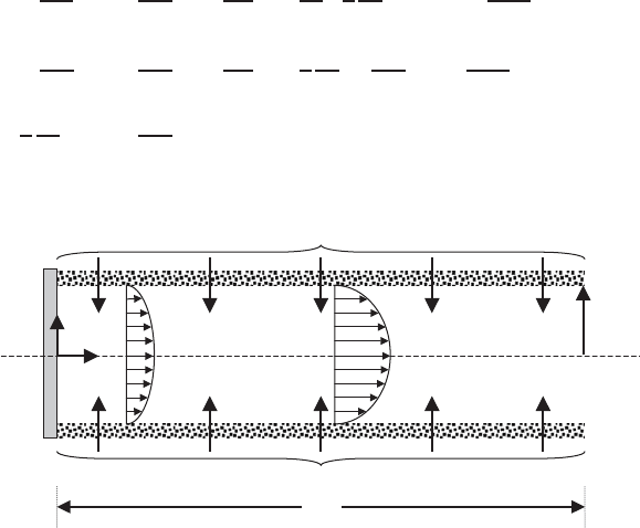
in a single ﬁber, as shown in Figure 3.E.10-1. Consider the case of a permeate

stream that consists of an incompressible Newtonian liquid with constant physical

properties. The ﬂow through the core (called the lumen) of the hollow ﬁber is

complex since the mass ﬂow increases as the permeate stream ﬂows toward the open

end. We use scaling analysis to explore the conditions under which the describing

equations for this ﬂow can be simpliﬁed.

The appropriately simpliﬁed equations of motion in cylindrical coordinates given

by equations (C.2-1), (D.2-10), and (D.2-12) in the Appendices along with the

boundary and auxiliary conditions are given by (step 1)

ρu

∂u

∂r

+ ρu

∂u

∂z

=−

∂P

∂r

+ μ

∂

∂r



∂

∂r

(ru

)



+ μ

∂

∂z

(3.E.10-1)

ρu

∂u

∂r

+ ρu

∂u

∂z

=−

∂P

∂z

+ μ

∂

∂r



∂u

∂r



+ μ

∂

∂z

(3.E.10-2)

∂

∂r

(ru

) +

∂u

∂z

= 0 (3.E.10-3)

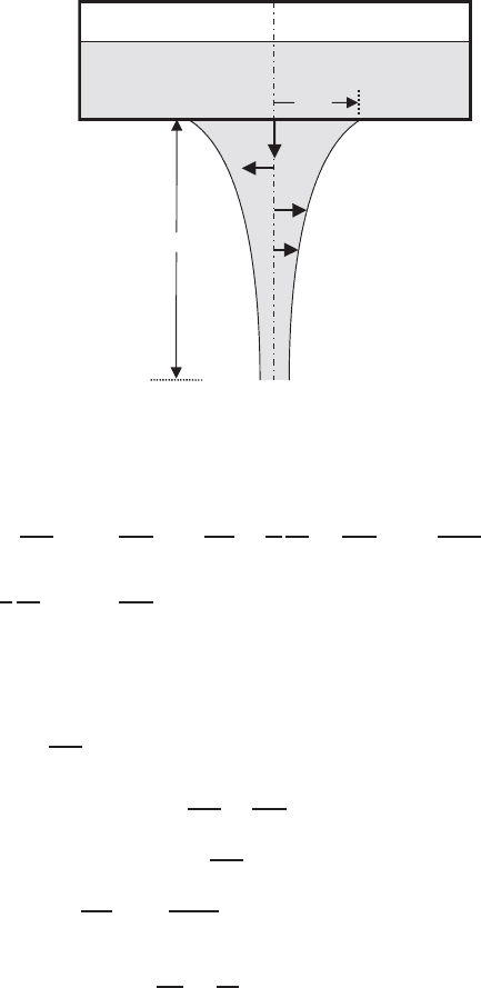
Figure 3.E.10-1 Flow of an incompressible Newtonian liquid in a cylindrical hollow-ﬁber

membrane of radius R, one end of which is closed and the other open, due to permeation

through the wall at a velocity U

; the axial velocity proﬁles shown at two axial positions

illustrate the acceleration caused by the mass addition due to the radial permeation.