Krantz W.B. Scaling Analysis in Modeling Transport and Reaction Processes: A Systematic Approach to Model Building and the Art of Approximation

Подождите немного. Документ загружается.

HEAT TRANSFER WITH PHASE CHANGE 173

Since L is merely some ﬁxed value of the axial coordinate x, the criteria above always

break down in the vicinity of the leading edge of the ﬂat plate. Hence, if one is seek-

ing to determine an integral quantity such as the total drag or heat ﬂux along the ﬂat

plate, the error will not be signiﬁcant if equations (4.6-36) and (4.6-37) are satisﬁed

over most of the plate. However, the error incurred by invoking the boundary-layer

approximation can be quite large in the vicinity of the leading edge of the plate for

point quantities such as the local velocity components, shear stress, temperature, or

heat ﬂux. Note for 90% of the ﬂat plate to satisfy the condition that Re ≥

◦

(100),

the Reynolds number at the end of the plate must be 1000. Since the Peclet number

is the product of the Reynolds number and the Prandtl number, equation (4.6-36) is

more limiting than equation (4.6-37) for ﬂuids other than liquid metals.

Note that scaling analysis suggests how a solution to the coupled heat- and

momentum-transfer problem can be developed that applies from the leading edge

of the plate to any arbitrary downstream distance. Recall that the coupled describing

equations are difﬁcult to solve, owing to the presence of the axial diffusion terms

in both the thermal energy equation and the equations of motion. These terms

require specifying downstream boundary conditions that in practice are usually not

known. However, the parabolic boundary-layer equations suggested by scaling can

be solved either numerically or via approximate analytical methods downstream

from the leading edge of the plate. The resulting solutions for the temperature and

velocity proﬁles then can be used as downstream boundary conditions on the full

elliptic describing equations that must be solved in the vicinity of the leading edge

of the ﬂat plate. Hence, we see that scaling not only provides a systematic method

for simplifying the describing equations, but also suggests a strategy for solving

them.

4.7 HEAT TRANSFER WITH PHASE CHANGE

Heat transfer is very often involved in problems wherein phase change occurs,

owing to the need to supply or remove the latent heat associated with the transition

from one phase to another. Figure 4.7-1 shows a schematic of melting ice within

porous soil that was initially at its freezing temperature T

and then was subjected

to a higher constant temperature T

at the ground surface. We will assume that

the heat transfer is one-dimensional and purely conductive and that the physical

properties are constant.

This example will illustrate scaling of a moving boundary

problem; that is, the melting front is a boundary that moves progressively downward

into the frozen soil as heat is conducted upward to the warm ground surface. We

will again explore how this problem can be simpliﬁed. We use this problem to

illustrate the forgiving nature of scaling by making a na

ıve mistake in the way we

Note that the melting of ice can induce free convection heat transfer arising from the density gradients

that can be generated, due to the fact that water has a density maximum at 4

◦

C; that is, unfrozen water

adjacent to melting ice is less dense than the water immediately above it, which can give rise to

free convection; however, this is not likely to occur in most soils, due to their low permeability to

ﬂow.

174 APPLICATIONS IN HEAT TRANSFER

L(t)

Frozen soil

Thawed soil

T = T

, t ≤ 0; T = T

, t > 0

T = T

Figure 4.7-1 Unsteady-state one-dimensional heat transfer due to the imposition of a tem-

perature T

at the surface of frozen water-saturated porous soil whose initial temperature was

where T

; the position of the thaw front denoted by L(t) progressively penetrates

farther into the frozen soil due to conductive heat transfer from the ground surface.

scale one of the derivatives. This will then lead to a contradiction that suggests

that we rescale the equations to achieve

◦

(1) scaling.

The describing equations are obtained by appropriately simplifying equation

(F.1-2) in the Appendices and prescribing the requisite initial and boundary condi-

tions (step 1):

∂T

∂t

= k

∂

∂x

(4.7-1)

T = T

at t = 0 (4.7-2)

T = T

at x = 0fort>0 (4.7-3)

T = T

at x = L(t) (4.7-4)

where k

,ρ

,andC

are the effective thermal conductivity, mass density, and

heat capacity, respectively, of the unfrozen soil; note that by effective we mean

that these properties account for the presence of the solid soil and the unfrozen

water that is contained in its pores. Equations (4.7-2) and (4.7-3) are the prescribed

initial temperature and imposed temperature at the ground surface, respectively.

Equation (4.7-4) states that ice and unfrozen water that meet at the freezing front are

in thermodynamic equilibrium at the freezing temperature of water. Note that this

boundary condition is applied at the moving interface between the ice and unfrozen

water L(t); hence, problems of this type are referred to as moving boundary prob-

lems.SinceL(t ) is an additional unknown, it is necessary to prescribe an auxiliary

condition to determine it. This is obtained via an integral energy balance as follows:



(T − T

◦

)dx +



∞

(T − T

◦

)dx = q

(4.7-5)

HEAT TRANSFER WITH PHASE CHANGE 175

where T

◦

is an arbitrary reference temperature for the enthalpy or heat content,

and C

are the effective mass density and heat capacity, respectively, of the

frozen soil, and q

is the heat transferred into the unfrozen soil at the ground surface.

Applying Leibnitz’s rule for differentiating an integral given by equation (H.1-2)

in the Appendices and substituting equation (4.7-1) while recalling that the frozen

ice remains at the constant temperature T

yields

(ρ

− ρ

)(T

− T

◦

)



∂

∂x

dx +



∞

∂

∂x

dx = q

(4.7-6)

The ﬁrst term in the above is the difference in heat content between the unfrozen

and frozen soil; this can be related to H

, the latent heat of fusion of water.

Hence, integrating equation (4.7-6) yields

H

ερ

+ k

∂T

∂x



x=L

− k

∂T

∂x



x=0

+ k

∂T

∂x



x=∞

− k

∂T

∂x



x=L

= q

(4.7-7)

where ρ

is the mass density of water, ε the porosity of the soil, and k

the thermal

conductivity of the frozen soil. The fourth and ﬁfth terms in equation (4.7-7) are

identically zero if there is no heat transfer in the frozen soil and the third term

is equal to the last term. Hence, the auxiliary condition needed to determine the

instantaneous location of the freezing front is given by

∂T

∂x

=−H

ερ

at x = L (4.7-8)

This condition merely states that the heat conducted to the freezing front supplies

the instantaneous latent heat required for melting the ice. To integrate equation

(4.7-8), it is necessary to specify an initial condition on L; this is given by

L = 0att = 0 (4.7-9)

Note that whenever boundary conditions must be applied at a location whose

position is unknown and dependent on the solution to the particular describing

equations, it is necessary to use some type of integral balance to obtain an addi-

tional condition to determine the location of this boundary. In ﬂuid dynamics this

occurs for ﬂows involving free surfaces such as were considered in Section 3.7

and Example Problem 3.E-8 and requires using an integral mass balance, which

is called the kinematic surface condition. In heat transfer this occurs in problems

such as the one considered here involving phase change and requires an integral

energy balance. In some heat-transfer problems involving phase change such as

evaporation, mass loss is also involved. In the latter moving boundary problems

it is necessary to include both an integral energy and an integral mass balance.

One of these is used as a boundary condition on the energy equation, and the

176 APPLICATIONS IN HEAT TRANSFER

other constitutes the auxiliary equation used to locate the position of the moving

boundary.

Deﬁne the following dimensionless dependent and independent variables (steps

2, 3, and 4):

∗

≡

T − T

; x

∗

≡

; t

∗

≡

; L

∗

≡

(4.7-10)

Introduce these dimensionless variables into the describing equations and divide

each equation through by the dimensional coefﬁcient of one term that should be

retained to maintain physical signiﬁcance (steps 5 and 6):

∂T

∗

∂t

∗

∂

∗

∂x

∗2

(4.7-11)

∗

− T

∗

= 0att

∗

= 0 (4.7-12)

∗

− T

at x

∗

= 0for t

∗

> 0 (4.7-13)

∗

− T

at x

∗

(4.7-14)

∂T

∗

∂x

∗



∗

=L/x

=−

H

εx

∗

at x

∗

(4.7-15)

∗

= 0att

∗

= 0 (4.7-16)

where α

= k

/ρ

is the thermal diffusivity of the unfrozen soil.

We can bound the dimensionless temperature to be

◦

(1) by setting the dimen-

sionless group in equation (4.7-12) or (4.7-14) equal to zero to determine the

reference temperature and by setting the dimensionless group in equation (4.7-13)

equal to 1 to determine the temperature scale (step 7); that is,

− T

= 0 ⇒ T

= T

;

− T

= 1 ⇒ T

= T

− T

(4.7-17)

We can bound the dimensionless spatial coordinate to be

◦

(1) by setting the dimen-

sionless group in equation (4.7-14) or (4.7-15) equal to 1; that is,

= 1 ⇒ x

= L

(4.7-18)

The time scale will again be the observation time t

since this is inherently an

unsteady-state problem. Since the two remaining terms in equation (4.7-15) must

balance each other, to ensure that each term is

◦

(1), we must set the dimensionless

HEAT TRANSFER WITH PHASE CHANGE 177

group in this equation equal to 1; this then provides the scale factor for the freezing

penetration front; that is,

H

εx

H

εL

− T

= 1 ⇒ L



− T

H



1/2

(4.7-19)

If we now rewrite our dimensionless describing equations in terms of the scales

deﬁned by equations (4.7-16) through (4.7-19), we obtain

− T

)

H

εα



∂T

∗

∂t

∗

−

∗

∂T

∗

∂x

∗



∂

∗

∂x

∗2

(4.7-20)

∗

= 0att

∗

= 0 (4.7-21)

∗

= 1atx

∗

= 0fort

∗

> 0 (4.7-22)

∗

= 0atx

∗

= 1 (4.7-23)

∗

=−

∗

at x

∗

= 1 (4.7-24)

Note that an additional term now appears in equation (4.7-20) because of the trans-

formation to a dimensionless spatial coordinate that is scaled with the instantaneous

depth of the thawed layer. This is referred to as a pseudo-convection term since it

involves a velocity multiplied by a spatial derivative in the same direction as that

of the velocity. Pseudo-convection terms will always arise when one transforms

from a stationary coordinate system to one for which either the reference or scale

factor is a function of time.

Now let us assess the conditions under which the dimensionless describing

equations can be simpliﬁed (step 8). We detect an immediate problem in

equation (4.7-20) in that the relative importance of the transformed unsteady-state

term is independent of the observation time t

. Recall from the problem consid-

ered in Section 4.3 that the unsteady-state term should be multiplied by the inverse

Fourier number, which is equal to the ratio of the observation time to the character-

istic heat conduction time. For very large Fourier numbers we would anticipate that

quasi-steady-state heat transfer should apply. Hence, we have obtained an unrea-

sonable result and the forgiving nature of scaling has indicated a contradiction:

namely, that quasi-steady-state conditions can never be achieved. Another contra-

diction inherent in this scaling is that the dimensionless thaw penetration depth is

always equal to 1 since L

∗

= L/L

= L/x

= 1. Therefore, we need to rescale the

problem; we will know that we have scaled correctly when the relevant terms are

bounded of

◦

(1) and no contradictions occur.

We suspect that our error was introduced by scaling dL/dt with L

.Let

us rescale the describing equations by introducing a scale factor

for dL/dt to

ensure that we bound this derivative to be

◦

(1):





∗

≡

(4.7-25)

178 APPLICATIONS IN HEAT TRANSFER

The other dimensionless variables are the same as deﬁned by equation (4.7-10).

Introduce these dimensionless variables into the describing equations and divide

each equation through by the dimensional coefﬁcient of one term that should be

retained to maintain physical signiﬁcance:

∂T

∗

∂t

∗

∂

∗

∂x

∗2

(4.7-26)

∗

− T

∗

= 0att

∗

= 0 (4.7-27)

∗

− T

at x

∗

= 0fort

∗

> 0 (4.7-28)

∗

− T

at x

∗

(4.7-29)

∂T

∗

∂x

∗

=−

H

εx





∗

at x

∗

(4.7-30)

Our reference and scale factors for the temperature, the time, and the spatial coor-

dinate remain the same as before. Since the two terms in equation (4.7-30) must

balance each other, to ensure that each term is

◦

(1), we must set the dimensionless

group in this equation equal to 1; this then provides the scale factor for the melting

front velocity; that is,

H

εx

H

εL

− T

)

= 1 ⇒

− T

)

H

εL

(4.7-31)

We see that L

never appears explicitly in our dimensionless describing equa-

tions. Hence, L can be nondimensionalized with any relevant length scale such

as the maximum thaw depth L

. If we now rewrite our dimensionless describing

equations in terms of the scales deﬁned by equations (4.7-17), (4.7-18), and (4.7-

31), we obtain

∂T

∗

∂t

∗

−

− T

)

H

∗





∗

∂T

∗

∂x

∗

∂

∗

∂x

∗2

(4.7-32)

∗

= 0att

∗

= 0 (4.7-33)

∗

= 1atx

∗

= 0fort

∗

> 0 (4.7-34)

∗

= 0atx

∗

= 1 (4.7-35)

∗

=−





∗

at x

∗

= 1 (4.7-36)

where Fo

≡ α

is the Fourier number for heat transfer. Note again that an

additional pseudo-convection term appears in equation (4.7-32), due to the trans-

formation from T(x,t) to T

∗

),inwhichx

∗

= x/L(t). The dimensionless

HEAT TRANSFER WITH PHASE CHANGE 179

group ρ

− T

)/H

ε multiplying the pseudo-convection term is a ratio

of the sensible heat to latent heat effects.

Now let us assess the conditions under which these dimensionless describing

equations can be simpliﬁed (step 8). We see that the relative importance of the

unsteady-state term in equation (4.7-32) is determined by the magnitude of the

Fourier number. The two terms in this equation must balance each other. We have

scaled ∂T

∗

/∂t

∗

to be

◦

(1). However, we are not certain that ∂

∗

/∂x

∗2

◦

(1).

The fact that we have scaled ∂T

∗

/∂x

∗

to be

◦

(1) does not necessarily ensure that

∂

∗

/∂x

∗2

◦

(1). If Fo

◦

(1), both the unsteady-state term and the conduction

term will be

◦

(1). This condition implies that

= 1 ⇒ L =

√

for short contact times (4.7-37)

The question might arise as to whether L

/α

can ever be much greater than 1,

corresponding to very short contact times. However, this would lead to a contra-

diction since the dimensionless unsteady-state term should be of the same order

as the dimensionless heat-conduction term. Hence, we conclude that for very short

contact times, L

∝ t

, to ensure that L

/α

remains bounded as t

→ 0; that is,

scaling analysis permits us to infer the time dependence of the thaw penetration

for short contact times.

Now let us consider the case when Fo

= α

 1, corresponding to very

long contact times. When this condition prevails, the unsteady-state term in equation

(4.7-32) can be ignored and quasi-steady-state prevails. The time dependence now

enters implicitly through both the pseudoconvection term and the condition applied

at the moving boundary given by equation (4.7-36). The resulting quasi-steady-

state describing equations can be solved analytically. However, if in addition

the dimensionless group multiplying the pseudo-convection term is small, that is,

− T

)/H

ε  1, further simpliﬁcation is possible. In the latter case,

equation (4.7-32) predicts a linear temperature proﬁle given by

∗

= 1 − x

∗

(4.7-38)

When equation (4.7-38) is substituted into equation (4.7-36) and the result is cast

into dimensional form and integrated, one obtains

− T

)

H

εL

= L

(4.7-39)

That is, for long contact times we ﬁnd that the solution to the describing equations

agrees identically with the scale factor for the thawing front velocity given by

equation (4.7-31). This should not be surprising since if scaling is done properly,

it should give estimates that are within an

◦

(1) factor of those obtained by solving

the describing equations. One can integrate equation (4.7-39) to obtain an equation

for L as a function of t;thatis,

− T

)

H

− t

) + L

for long contact times (4.7-40)

180 APPLICATIONS IN HEAT TRANSFER

where L

is an integration constant; note that one cannot apply the initial condition

that L = 0 since equation (4.7-40) does not apply at short times. However, this

initial condition can be estimated from the short-time solution given by equation

(4.7-37). Note also that although both equations (4.7-37) and (4.7-40) predict that

will increase linearly with t

, the short-contact time thaw-penetration rate is

faster than that for the long-contact time.

In summary, if Fo

 1, this unsteady-state moving boundary heat-transfer

problem can be considered to be quasi-steady-state; that is, the describing

equations can be simpliﬁed by ignoring the unsteady-state term in the thermal

energy equation. For quasi-steady-state conditions the time dependence enters

through the boundary condition at the moving boundary whose location is time-

dependent.

4.8 TEMPERATURE-DEPENDENT PHYSICAL PROPERTIES

In Section 3.9 we used scaling analysis to determine when the incompressible ﬂow

assumption could be made for a ﬂuid whose density was pressure-dependent. Here

we consider a related coupled ﬂuid-dynamics and heat-transfer problem in which

we will use scaling to determine when the temperature-dependent shear viscosity

can be assumed to be constant. Note that the manner in which scaling analysis is

used to assess when the temperature-dependence of the viscosity can be ignored

in this problem can be applied to assessing when the dependence of any other

physical or transport property on some state variable such as temperature, pressure,

or concentration can be ignored.

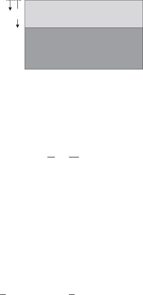
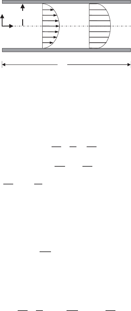
Figure 4.8-1 shows a schematic of the steady-state pressure-driven ﬂow of an

incompressible Newtonian liquid between two inﬁnitely wide parallel ﬂat plates,

each of which is maintained at T

, which is also the initial temperature of the

liquid. The shear ﬂow causes signiﬁcant viscous heating that can possibly cause

a progressive decrease in the liquid viscosity whose temperature dependence is

given by

μ = Ae

B/T

(4.8-1)

where A and B are positive constants. This in turn implies a possible developing

ﬂow due to the inﬂuence of the decrease in viscosity on the velocity proﬁle. How-

ever, we will invoke the lubrication-ﬂow

and low Peclet number approximations

and in addition ignore axial conduction.

We use scaling analysis to assess when

the temperature dependence of the viscosity can be ignored.

Appropriate simpliﬁcation of the equations of motion given by equations (D.1-

10) and (D.1-11) in the Appendices and the thermal energy equation given by

Scaling analysis was applied to justify the lubrication-ﬂow approximation in Section 3.3.

Scaling analysis was applied to justify the low Peclet number approximation, ignoring the axial

conduction in Section 4.5.

TEMPERATURE-DEPENDENT PHYSICAL PROPERTIES 181

Figure 4.8-1 Steady-state pressure-driven lubrication ﬂow of an incompressible Newtonian

liquid between two inﬁnitely wide parallel ﬂat plates, each of which is maintained at T

which is also the initial temperature of the liquid; this shear ﬂow causes viscous heating

that can result in a progressive decrease in the liquid viscosity; representative velocity and

temperature proﬁles are shown in this ﬁgure.

equation (F.1-2), and speciﬁcation of the required boundary conditions yields the

following set of describing equations (step 1):

0 =

P





(4.8-2)

0 = k

+ μ





(4.8-3)

= 0,

= 0aty = 0 (4.8-4)

= 0,T= T

at y =±H (4.8-5)

Since we seek to assess when the temperature dependence of the viscosity can be

ignored, we need consider only small departures of the temperature from the initial

temperature T

. Hence, it is convenient to expand equation (4.8-1) in a Taylor series

about T

at which the viscosity is μ

μ = μ

−

Bμ

(T − T

) +

◦

(T − T

)

(4.8-6)

Since we need consider only the ﬁrst-order effects of temperature to assess whether

there is any signiﬁcant change in the viscosity, truncate equation (4.8-6) after the

second term on the right-hand side and substitute it into equations (4.8-2) and

(4.8-3):

0 =

P

−

Bμ

(T − T

)

(4.8-7)

182 APPLICATIONS IN HEAT TRANSFER

0 = k

−

Bμ

(T − T

)





(4.8-8)

Introduce the following scale and reference factors (steps 2, 3, and 4):

∗

≡

; T

∗

≡

T − T

; x

∗

≡

; y

∗

≡

(4.8-9)

Substitute these dimensionless variables into the describing equations and divide

each equation through by the dimensional coefﬁcient of one term that should be

retained in order to maintain physical signiﬁcance (steps 5 and 6):

0 =

P

∗

1 −



∗

− T



∗

(4.8-10)

0 =

∗

∗2

1 −



∗

− T





∗



(4.8-11)

∗

= 0,

∗

= 0aty

∗

= 0 (4.8-12)

∗

= 0,T

∗

− T

at y

∗

=±

(4.8-13)

When set equal to zero and 1, respectively, the dimensionless groups in equations

(4.8-13) provide the following reference and scale factors (step 7):

− T

= 0 ⇒ T

= T

= 1 ⇒ y

= H (4.8-14)

Since the pressure term must balance the principal viscous term for this lubrication

ﬂow, the dimensionless pressure term in equation (4.8-10) must be set equal to 1

to obtain the velocity scale:

P

= 1 ⇒ u

P

(4.8-15)

This is a reasonable velocity scale since it is equal to the average velocity for

fully developed laminar ﬂow between two parallel ﬂat plates. Since the viscous

dissipation must be balanced by the heat conduction to the parallel ﬂat plates, the

dimensionless dissipation term in equation (4.8-11) must be set equal to 1 to obtain

the temperature scale:



P



= 1 ⇒ T

kμ



P



(4.8-16)