Kusse B.R., Westwig E.A. Mathematical Physics: Applied Mathematics for Scientists and Engineers
Подождите немного. Документ загружается.

186
INTRODUCTION
TO
COMPLEX
VARIABLES
Example
6.12
Let's
evaluate
1
I-€
1
pps_:dx
(x2
+
l)(x
-
1)
=
!"o
{
L
dx
(x2
+
I)(x
-
1)
.
(6.238)
1
+
Jli,
dx
(x2
+
l)(x
-
1)
Applying the above arguments,
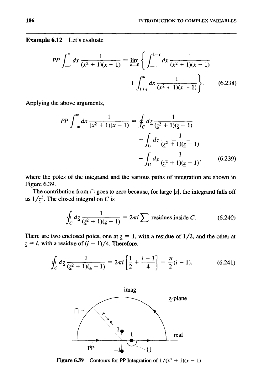
where the poles of the integrand and the
various
paths of integration
Figure 6.39.
(6.239)
are shown in
-
The contribution from
fl
goes to zero because,
for
large
lzl,
the integrand falls
off
as
1
/z3.
The
closed integral
on
C
is
1
=
2m residues inside
C.
(6.240)
There are two enclosed poles, one at
g
=
1, with a residue
of
1
/2, and
the
other at
z
=
i,
with a residue of
(i
-
1)/4.
Therefore,
imag
-
z-plane
real
Figure
639
Contours
for
PP
Integration
of
I
/(x2
+
l)(x
-
1)
DEFINITE INTEGRALS
AND
CLOSURE
187
imag
'0
-
z-plane
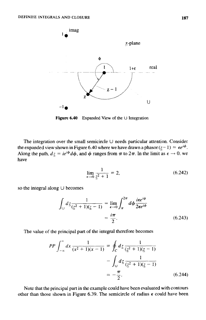
Figure
6.40
Expanded
View
of
the
U
Integration
The integration over the small semicircle
U
needs particular attention. Consider
the expanded view shown in Figure
6.40
where we have drawn a phasor
(g-
1)
=
Eei4.
Along the path,
dg
=
ie'@d+,
and ranges
from
IT
to 2~.
In
the limit as
E
+
0,
we
have
1
lim
-
=
2,
E'O
22
+
1
so
the integral along
U
becomes
irr
2
-
-_
The value
of
the principal part
of
the integral therefore becomes
1
1
(x2
+
l)(x
-
1)
PP
1;
d.r
IT
-_
- -
2'
(6.242)
(6.243)
(6.244)
Note that the principal part in the example could have been evaluated with contours
other than
those
shown in Figure
6.39.
The semicircle
of
radius
E
could have been
188
INTRODUCTION
TO
COMPLEX
VARIABLES
taken above the singularity at
g
=
1,
and/or the infinite
radius
contour could have
been placed in the lower half of the 2-plane. The result obtained for the principal part
of
the integral is the same with any of these choices.
6.11.5 Definite
Integrals
with
sin
8
and
cos
8
Real integrals of the form
r2a
I
=
J,
do
w(sin
8,
cos
e),
(6.245)
where the integrand is a function of sin
8
and cos
8,
can sometimes be converted to
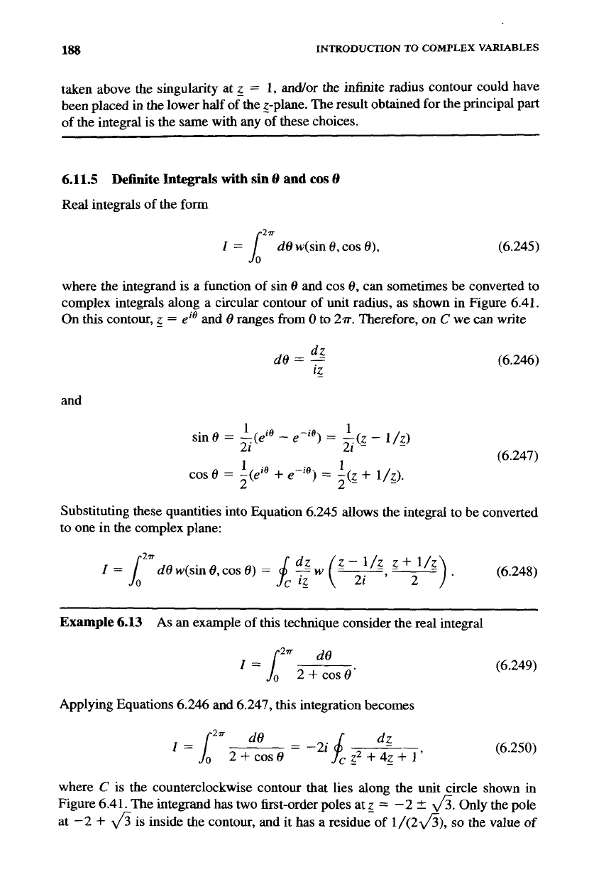
complex integrals along
a
circular contour of unit radius, as shown in Figure 6.41.
On
this
contour,
g
=
eie
and
6
ranges
from
0
to 2v. Therefore,
on
C
we
can write
(6.246)
and
sine
=
L(eie
-
e-ie)
=
-(z 1
-
1/g)
1
ie
1
cos
e
=
-(e
+
e+’)
=
2(g
+
1/g).
Substituting these quantities into Equation 6.245 allows the integral to be converted
to one in the complex plane:
(6.247)
2i
2i
-
2
Example
6.13
As
an example of
this
technique consider the real integral
d6
2“
I=I
2+COS6’
Applying Equations 6.246 and 6.247,
this
integration becomes
(6.249)
(6.250)
where
C
is the counterclockwise contour that lies along the unit circle shown in
Figure 6.41. The integrand has two first-order poles at
g
=
-2
*
&.
Only the pole
at
-2
+
&
is inside the contour, and it has
a
residue of 1/(2&),
so
the value
of
CONFORMAL MAPPING
189
,
imag
I
-
z-plane
Figure
6.41
Contour
for
Real
sin,
cos
Integrals
the integral becomes
=2m(s)
(6.251)
(6.252)
6.12
CONFORMAL
MAPPING
Conformal Mapping is a technique for finding solutions to Laplace’s equation in
two dimensions. These solutions are of interest in fluid mechanics and electro- and
magnetostatics.
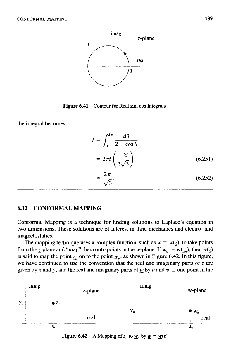
The mapping technique uses a complex function, such
as
w
=
I&),
to take points
from the Z-plane and “map” them onto points in the w-plane.
If
4210
=
y(~),
then
y(z)
is
said to map the point on to the point
%,
as shown in Figure
6.42.
In
this
figure,
we have continued to use the convention that the real and imaginary parts of
z
are
given by
x
and
y,
and the real and imaginary parts of
w
by
u
and
u.
If
one point in the
~
I
imag
w-plane
z-plane
imag
Yo
I
0
2,
I
vo
real
-*
W”
real
Figure
6.42
A
Mapping
of
z,
to
%
by
w
=
w(z)
190
INTRODUCTION
TO
COMPLEX VARIABLES
g-plane maps to only one point in the w-plane, the mapping function
&)
is said
to
be
single valued. It is possible for the mapping function
to
take one point in the Z-plane
to more than one point in the w-plane.
This
type
of
function is called multivalued.
Mapping is
a
two-way street. The function
~(g)
can
be
inverted to give a function
of
w,
i.e.,
go,
that takes points from the w-plane
and
maps them back to points in
the z-plane.
If
both
~(g)
and
ZW
are single valued, the mapping between the two
complex planes is called ‘‘oneto one:’
6.12.1
Mapping
of
Grid
Lines
Many
times it is easier
to
discuss mapping properties with the use of a specific
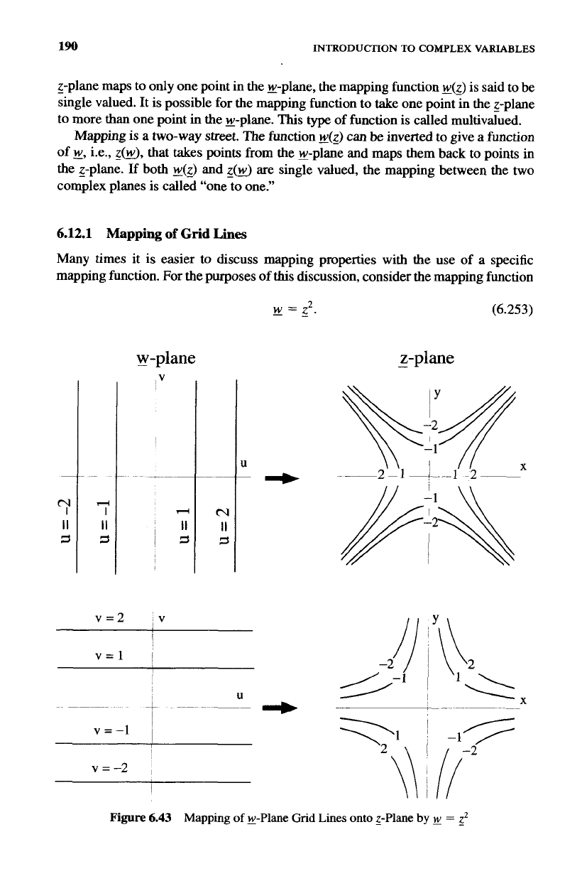
mapping function. For the purposes of
this
discussion, consider
the
mapping function
w-plane
N
I1
a
2
-
w=g.
-
z-plane
(6.253)
v=2
,v
v=l
~
I
v
=
-2
Figure
6.43
Mapping
of
E-Plane
Grid
Lines onto z-Plane
by
w
=
g2
CONFORMAL
MAPPING
191
-plane
X
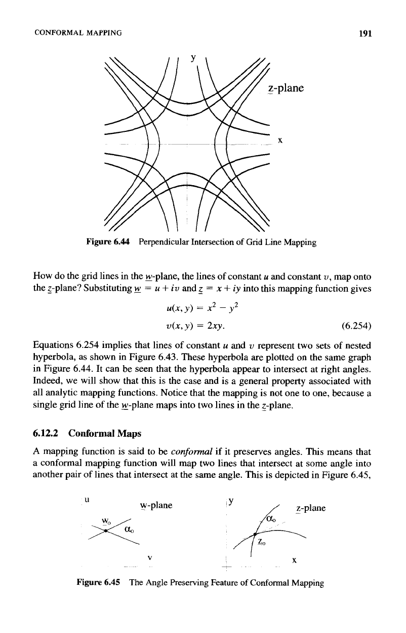
Figure
6.44
Perpendicular Intersection
of
Grid Line Mapping
How do the grid lines in the w-plane, the lines of constant
u
and constant
u,
map onto
the Z-plane? Substituting
441
=
u
+
iv
and
=
x
+
iy
into
this
mapping function gives
u(x,
y)
=
x2
-
y2
v(x,y)
=
2xy.
(6.254)
Equations 6.254 implies that lines of constant
u
and
u
represent two sets of nested
hyperbola, as shown in Figure 6.43. These hyperbola are plotted on the same graph
in Figure 6.44. It can be seen that the hyperbola appear to intersect at right angles.
Indeed, we will show that this is the case and is a general property associated with
all analytic mapping functions. Notice that the mapping is not one
to
one, because
a
single grid line
of
the w-plane maps into
two
lines in the Z-plane.
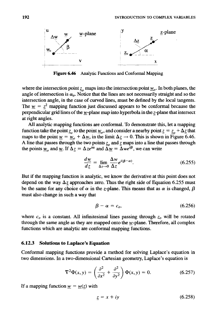
6.12.2
Conformal
Maps
A
mapping function is said to be
conformal
if it preserves angles. This means that
a conformal mapping function will map two lines that intersect at some angle into
another pair of lines that intersect at the
same
angle. This is depicted in Figure 6.45,
u
1
w-plane
/
1'"
z-plane
IY
u
w-plane
I
X
V
-
Figure
6.45
The
Angle
Preserving Feature
of
Conformal Mapping
192
INTRODUCTION TO
COMPLEX VARIABLES
V
-
X
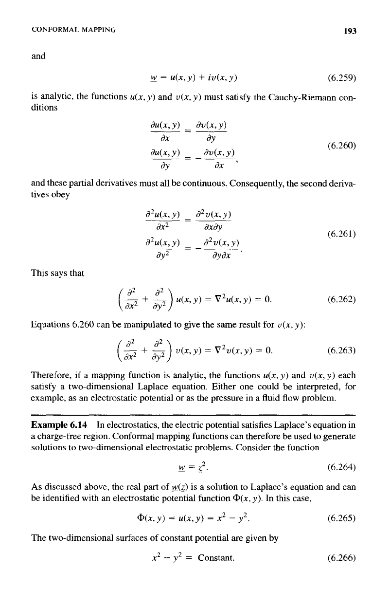
Figure
6.46
Analytic
Functions
and
Conformal
Mapping
where the intersection point
z,
maps into the intersection point
w-.
In
both planes, the
angle of intersection is
ao.
Notice that the lines are not necessarily straight and
so
the
intersection angle, in the case of curved lines, must
be
defined by the local tangents.
The
w
=
g2
mapping function just discussed appears to
be
conformal because the
perpendicular grid lines of the g-plane map into hyperbola in the z-plane that intersect
at right angles.
All analytic mapping functions
are
conformal.
To
demonstrate
this,
let a mapping
function take the point
z,
to the point
w+,,
and consider
a
nearby point
z
=
~0
+
Ag
that
maps to the point
g
=
w-
+
Aw,
in the limit
Az
-+
0.
This
is shown in Figure 6.46.
A line that passes through
the
two
points
z,
and
g
maps into a line that passes through
the points
w-
and
g.
If
Ag
=
AzeiU
and
AE
=
Awe'P,
we can write
(6.255)
But
if
the
mapping function is analytic, we know the derivative at
this
point does not
depend on
the
way
Az
approaches zero.
Thus
the right side of Equation 6.255 must
be the same
for
any choice
of
a
in the z-plane.
This
means that as
a
is changed,
p
must also change in such a way that
p
-
a
=
c,,
(6.256)
where
c,
is a constant. All infinitesimal lines passing through
zo
will be rotated
through
the
same
angle
as
they are mapped onto the E-plane. Therefore, all complex
functions which are analytic
are
conformal mapping functions.
6.12.3
Solutions
to
Laplace's
Equation
Conformal mapping functions provide a method for solving Laplace's equation in
two dimensions.
In
a two-dimensional Cartesian geometry, Laplace's equation is
V2@(x,
y)
=
(2
+
$)
@(x,
y)
=
0.
If
a mapping function
w
=
~(g)
with
(6.257)
g=x+iy
(6.258)
CONFORMAL MAPPING
and
193
-
w
=
u(x, y)
+
iv(x,
y)
(6.259)
is analytic, the functions
u(x,
y)
and
v(x,
y)
must satisfy the Cauchy-Riemann con-
ditions
(6.260)
and these partial derivatives must all be continuous. Consequently, the second deriva-
tives obey
This says that
(5
+
$)
u(x, y)
=
V2u(x, y)
=
0.
Equations 6.260 can be manipulated
to
give the same result for
v(x,
y):
($
+
$)
v(x, y)
=
V2v(x,
y)
=
0.
(6.261)
(6.262)
(6.263)
Therefore,
if
a mapping function is analytic, the functions
u(x,
y)
and
v(x,
y)
each
satisfy a two-dimensional Laplace equation. Either one could be interpreted, for
example, as an electrostatic potential
or
as the pressure in a fluid flow problem.
Example
6.14
In electrostatics, the electric potential satisfies Laplace’s equation in
a charge-free region. Conformal mapping functions can therefore be used
to
generate
solutions to two-dimensional electrostatic problems. Consider the function
(6.264)
-
w=z.
As
discussed above, the real part
of
I&)
is
a
solution
to
Laplace’s equation and can
be identified with an electrostatic potential function
@(x, y).
In this case,
2
@(x,
y)
=
u(x,
y)
=
x2
-
y2.
(6.265)
The two-dimensional surfaces of constant potential are given by
x2
-
y2
=
Constant.
(6.266)
194
INTRODUCTION
TO
COMPLEX
VARIABLES
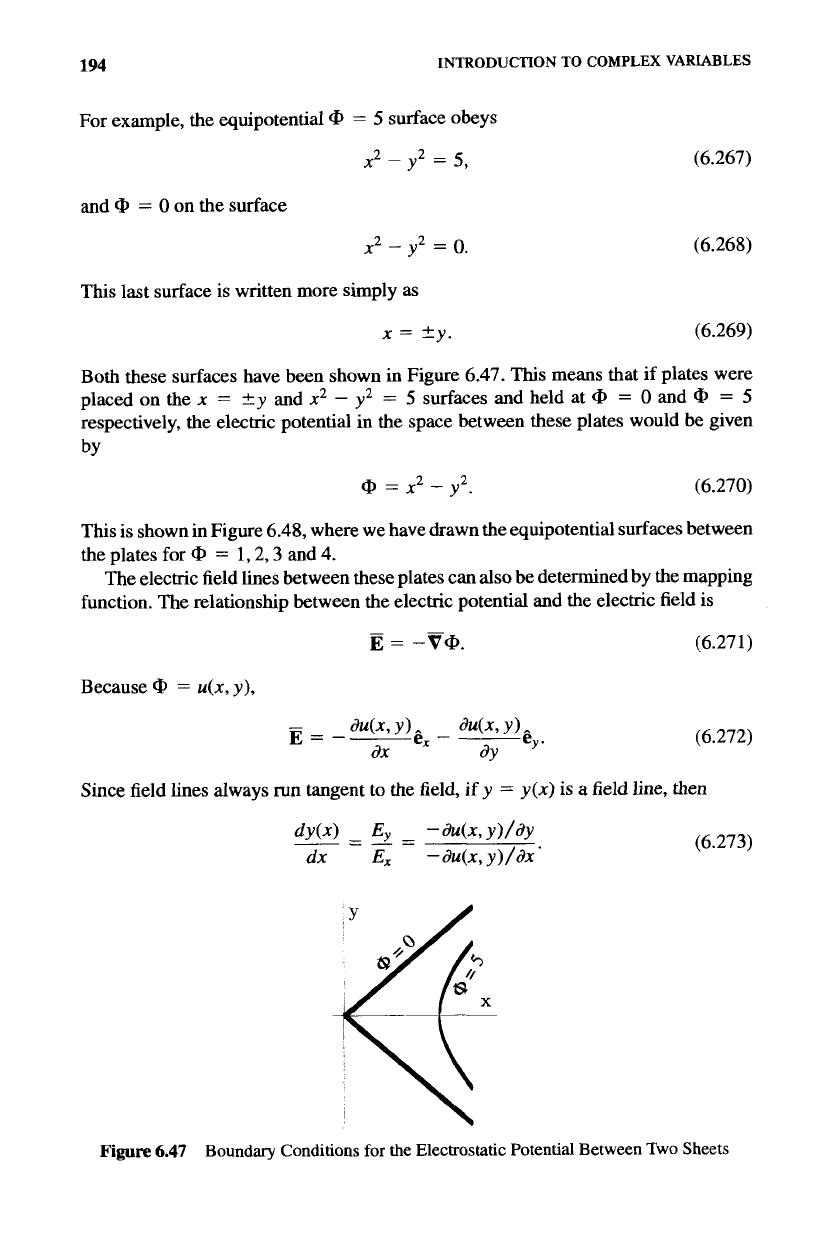
For example, the equipotential
Q,
=
5
surface obeys
x2
-
y2
=
5,
and
@
=
0
on the surface
x2
-
y2
=
0.
This
last surface is written more simply as
x
=
2y.
(6.267)
(6.268)
(6.269)
Both these surfaces have been shown
in
Figure 6.47.
This
means that if plates were
placed on the
x
=
?y
and
x2
-
y2
=
5
surfaces and held at
=
0
and
=
5
respectively, the electric potential
in
the space between these plates would be given
by
@
=
x2
-
y2.
(6.270)
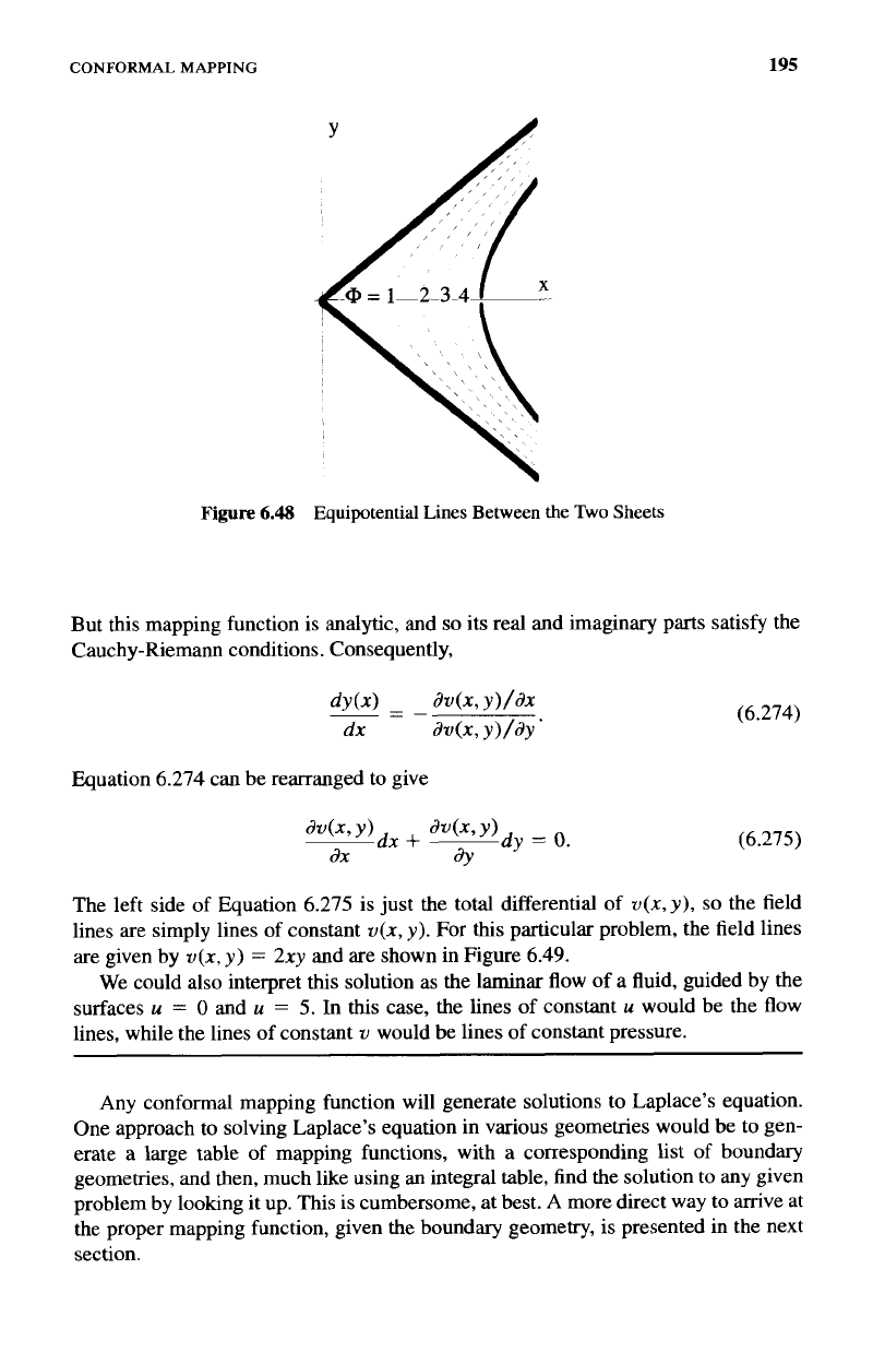
This
is
shown in Figure
6.48,
where we have drawn the equipotential surfaces between
the plates for
@
=
1,2,3 and 4.
The electric field lines between these plates can
also
be determined by the mapping
function. The relationship between
the
electric potential and the electric field is
-
E
=
-V@.
(6.271)
Because
Q,
=
u(x,
y),
(6.272)
Since field lines always run tangent
to
the field,
if
y
=
y(x)
is a field line, then
(6.273)
Figure
6.47
Boundary Conditions
for
the Electrostatic Potential Between
Two
Sheets
CONFORMAL
MAPPING
195
Figure
6.48
Equiptentid Lines Between the
Two
Sheets
But this mapping function is analytic, and
so
its real and imaginary parts satisfy the
Cauchy-Riemann conditions. Consequently,
Equation
6.274
can be rearranged to give
(6.274)
(6.27
5)
The left side of Equation
6.275
is just the total differential of
v(x,y),
so
the field
lines are simply lines of constant
v(x,
y).
For this particular problem, the field lines
are given by
v(x,
y)
=
2xy
and are shown in Figure
6.49.
We could also interpret
this
solution as the laminar flow of a fluid, guided by the
surfaces
u
=
0
and
u
=
5.
In
this case, the lines of constant
u
would be the flow
lines, while the lines of constant
v
would be lines of constant pressure.
Any
conformal mapping function will generate solutions to Laplace’s equation.
One approach to solving Laplace’s equation in
various
geometries would be to gen-
erate a large table of mapping functions, with a corresponding list of boundary
geometries,
and
then, much like using an integral table, find the solution to any given
problem by looking it up. This is cumbersome, at best.
A
more direct way to anive at
the proper mapping function, given the boundary geometry, is presented in the next
section.