Kusse B.R., Westwig E.A. Mathematical Physics: Applied Mathematics for Scientists and Engineers
Подождите немного. Документ загружается.

166
INTRODUCTION
TO
COMPLEX
VARIABLES
the
n
2
0
terms diverge outside the singularity circle that passes through
&.
The
combination only converges between the two singularity circles.
The
Contour
C
Out3ide
the
Large
Singu-
Circle
As
a
final
variation on
this
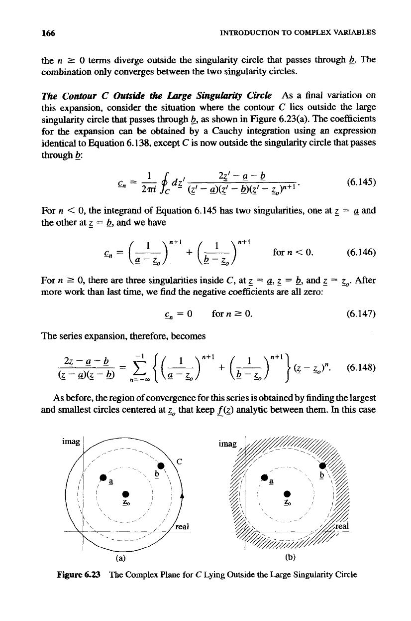
expansion, consider the situation where the contour
C
lies outside the large
singularity circle that passes through
b,
as
shown
in
Figure 6.23(a). The coefficients
for the expansion can
be
obtained
by a Cauchy integration using
an
expression
identical to Equation 6.138, except
C
is
now outside the singularity circle that passes
through
b:
(6.145)
For
n
<
0,
the integrand of Equation 6.145 has two singularities, one at
z
=
a
and
the other at
z
=
b,
and we have
n+l
n+l
.=(=)
+(=)
forn<O. (6.146)
For
n
2
0,
there are three singularities inside
C,
at
2
=
a,
z
=
b,
and
g
=
L.
After
more work than last time, we find the negative coefficients are all zero:
4
=
0
forn
2
0.
(6.147)
The series expansion, therefore, becomes
As
before,
the
region of convergence for
this
series is obtained by finding the largest
and smallest circles centered at
z,
that keep
f(z)
analytic between them.
In
this case
-
(4
Figure
6.23
The Complex Plane
for
C
(b)
Lying
Outside
the
Large Singularity Circle
THE COMPLEX LAURENT SERIES
167
the smallest circle lies just outside the singularity circle that passes through
z
=
b.
The largest circle can be extended to infinity because there are no other nonanalytic
points of
f(z_).
Therefore, the convergence region is
as
shown in Figure
6.23(b).
In thiscase we again obtain a true Laurent series. The coefficients of the series
contain two terms. The first generates a Laurent series for l/(z
-
a)
and the second
a Laurent series for 1
/(z
-
b).
The 1
/(z
-
uJ
part of the series converges outside the
singularity circle that passes through
a.
The
1
/(g
-
bJ
part of the series converges out-
side the singularity circle that passes through
b.
The combination converges outside
the largest of the two singularity circles, the one passing through
b.
6.9.2
Laurent Coefficients
Using
the Basic
Taylor
Series
Evaluating series coefficients from Equation 6.136 is not always
an
easy
task.
For-
tunately, like the Taylor series, Laurent series often
can
be generated from the basic
series expansion of Equation 6.100.
This
is best demonstrated by an example.
Example
6.8
Consider the function
(6.149)
1
Z-a
-
f(z>
=
-9
which is analytic at every point except
function expanded about
5
=
0
in the form
=
a.
We seek a Laurent series for this
(6.150)
We can manipulate Equation 6.149 using Equation 6.100 to obtain
L=(;)(&-)=(~)[l+;+(Q)2+-.]
z-a
(6.151)
This is in the form of a Laurent series with
only
n
<
0
terms. The coefficients
of
Equation 6.150 are
0
nrO
Cn
=
{
-
a-"-'
n<O'
Because the series expansion in Equation 6.150 converges if
lzl
>
lal,
(6.152)
(6.153)
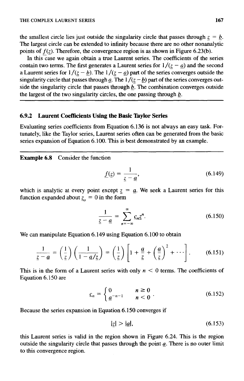
this Laurent series is valid in the region shown in Figure 6.24. This is the region
outside the singularity circle that passes through the point
a_.
There
is
no outer limit
to this convergence region.
168
INTRODUCTION
TO
COMPLEX VARIABLES
Figure
6.24
Convergence Region for Laurent Series Expansion About
5
=
0
The procedure for an expansion about an arbitrary point
z
=
z,
is similar. Manip-
ulate Equation 6.149
as
1
-
1
--
z-g
(z-z,)-@-z,)
1
(6.154)
Expanding the second term gives
1
I+=---+
a-%
(-,:+...I.
a-z,
z-z,
z-z,
which again is
a
Laurent series with coefficients
0
n20
=
{
(a
-
%)-n-l
n
<
0
*
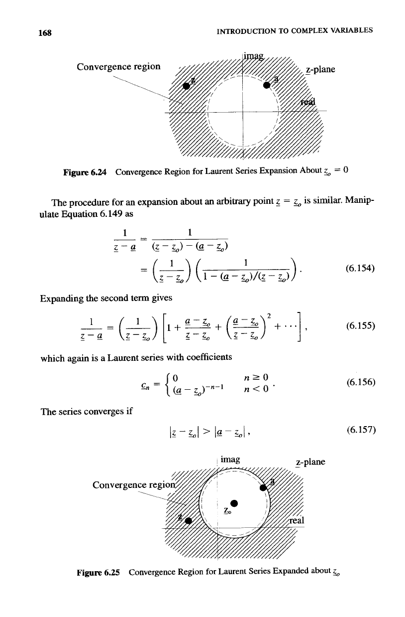
The series converges if
Iz
-
51
’
la
-
51
7
imag
z-plane
Convergence regio
1
(6.155)
(6.156)
(6.157)
Figure
6.25
Convergence Region for Laurent Series Expanded about
z,
THE
COMPLEX
LAURENT
SERIES
169
which is a region outside the singularity circle centered at
z,
and passing through
-
a,
as shown in Figure 6.25. Notice, the region of convergence can
be
modified by
changing the expansion point
5.
As
z,
gets closer to
a,
the series becomes valid for
more and more of the complex plane, but can never be made to converge exactly at
z
=
a.
-
6.9.3 Classification
of
Singularities
Laurent expansions allow singularities of functions to
be
categorized. Imagine the
point
z
=
a
is a singularity of the function
f(3.
If the most negative term in the
Laurent series expansion around the singular &int is
-m,
the singularity is called a
pole
of order
m.
For example, the function
(6.158)
is its own Laurent expansion around
z
=
a,
and thus this function has a pole of order
one at that point. This is often calleda simple pole. The function
(6.159)
1
f(z>
=
~
-
(z
-
d3
again is its own Laurent Expansion around
z
=
three.
nation does not. An example is the function
and therefore has a pole of order
It is possible to have a function that appears to have a pole, but on closer exami-
(6.160)
This function has a singularity at the point
g
=
0,
because the denominator goes
to
zero, but the Laurent expansion around
z
=
0
has no negative terms. This type of
singularity is called
removable
because the function does not diverge as we approach
the singularity. This can be seen in the case of Equation 6.160 because
(6.161)
even though the value exactly at
z
=
0
is undefined.
It was quite easy
to
determine the order of
the
singularities in Equations 6.158 and
6.159, because they were in the convenient form of 1/(g
-
d)".
For
a singularity
of
a more complicated function, you might
think
we would always have to determine
the coefficients of the Laurent series. Fortunately, there is another approach, which is
often much quicker. Notice for
a
pole
of
order
m
at
z
=
a,
multiplication by the factor
(z
-
a)"
will get rid of the divergence at
a.
In
other words, if the original function
170
INTRODUCTION TO COMPLEX
VARIABLES
diverges because of
a
pole of order
rn
at
z
=
a,
i.e.,
the divergence can be removed by multiplying by the factor
(z
-
UJ""
lim
[f(g)(z
-
d,"]
-+
a finite value.
(6.163)
z-%?
Thus, one way to determine
the
order of a pole is to multiply by successive factors
of
(z
-
13),
until
the result
no
longer diverges at
a.
The number of multiplying factors
needed determines the order of the pole.
and
this
diver-
gence cannot
be
removed by multiplying by
(z
-
uJm
for
any
value
of
m.
This
is called
an
essential
singularity. The Laurent expansion for a function about an essential sin-
gularity point will have an infinite number of negative
n
terms. The function
e
''2
has
an essential singularity at
z
=
0.
This
function goes to infinity at
z
=
0
faster than
any power of
g
goes to
0.
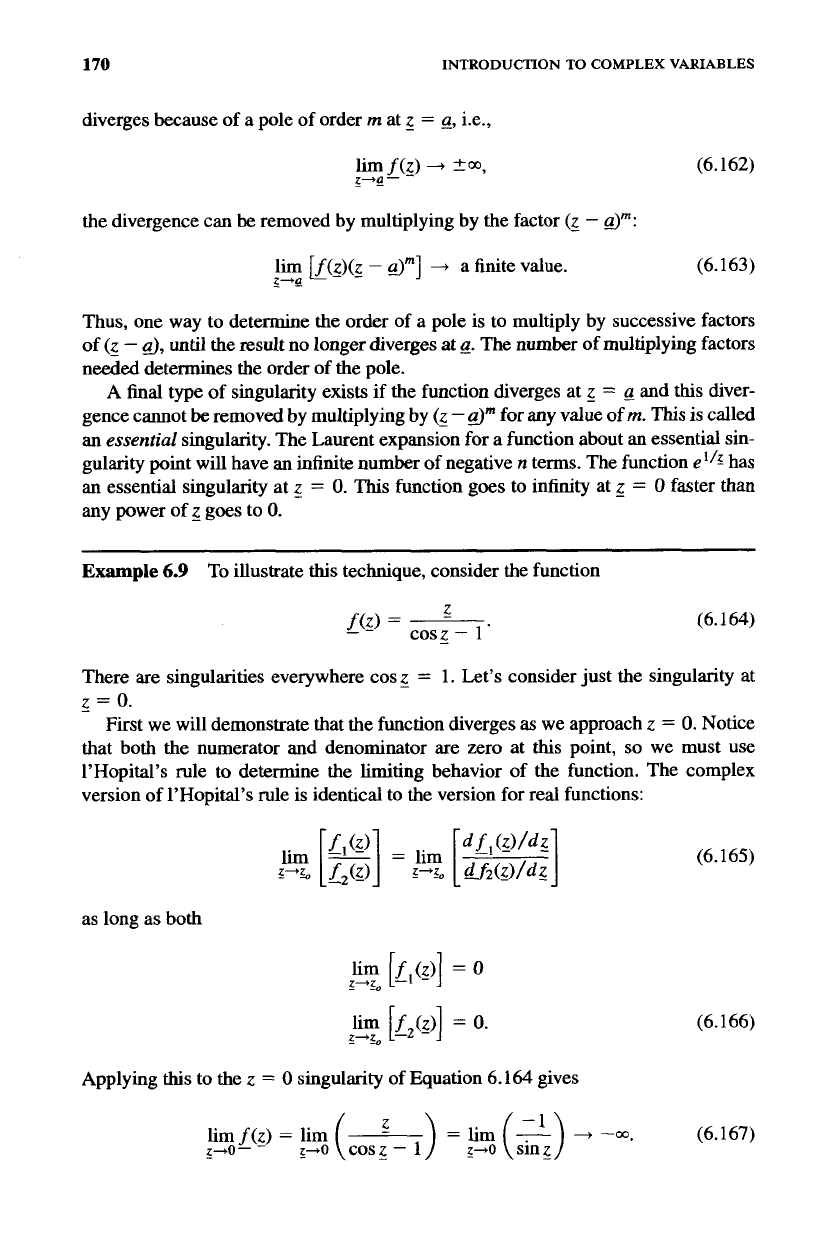
A final type of singularity exists if the function diverges at
z
=
Example
6.9
To illustrate
this
technique, consider the function
(6.1
64)
There are singularities everywhere cos
z
=
1. Let's consider just the singularity at
z
=
0.
First we will demonstrate that the function diverges
as
we approach
z
=
0.
Notice
that both the numerator and denominator
are
zero at this point,
so
we must use
1'Hopital's rule
to
determine the limiting behavior of the function. The complex
version of 1'Hopital's rule is identical to the version for red functions:
as long
as
both
lim
f
(z)
=
0
lim
[f
(z)]
=
0.
%-I,
[I
-1
-
5'1
-2
-
Applying
this
to the
z
=
0
singularity of Equation 6.164 gives
(6.165)
(6.166)
lim
f(z)
=
lim
(
z
)
=
lim
(2)
-+
-m.
(6.167)
240
-
2-+0
cosz
-
1
g+o
THE
RESIDUE
THEOREM
171
Now let's determine the order
of
the pole. Start by multiplying the function by
g
and taking the limit:
(6.168)
To
determine this limit, use 1'Hopital's rule:
not once, but twice:
Multiplying
by
z
has removed the divergence,
so
the singularity at
z
=
0
is a pole
of
order one.
6.10
THE RESIDUE THEOREM
It could be argued that the most useful result
of
this chapter is the Residue Theorem.
This theorem provides a powerful tool for calculating both complex contour integrals
and real, definite integrals.
6.10.1
Consider
an
integral
of
%(I)
on
an
arbitrary closed contour in the Z-plane:
The Residue
of
a
Single Pole
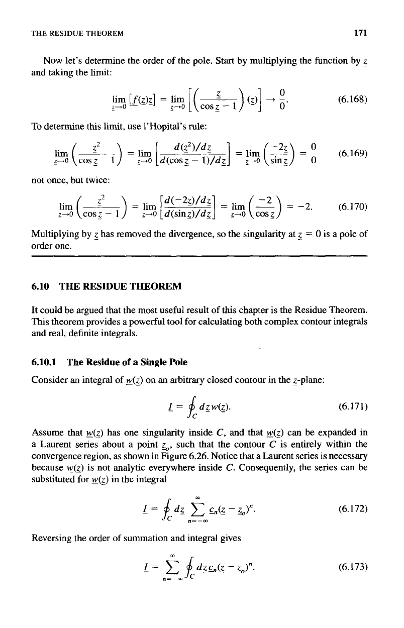
Assume that
y(z)
has one singularity inside
C,
and that
~(g)
can be expanded in
a Laurent series about a point
G,
such that the contour
C
is entirely within the
convergence region, as shown in Figure 6.26. Notice that a Laurent series is necessary
because
&)
is not analytic everywhere inside
C.
Consequently, the series can be
substituted for
~(z)
in the integral
m
Reversing the order
of
summation and integral gives
(6.172)
(6.173)
172
INTRODUCTION TO
COMPLEX
VARIABLES
Figure
6.26
Contour
and
Convergence
Annulus
for Residue Theorem
Integration
Consider any one of the terms with
n
2
0.
Its contribution to
I
must
be
zero
because the integrand is analytic everywhere:
Now
look
at the
n
=
-2
term. According
to
Cauchy’s Integral Formula,
(6.174)
(6.175)
so the contribution of
this
term to
I
is also zero.
This
will be the case for all terms of
the series with
n
5
-2.
For
n
=
-
1, however,
(6.176)
where again, the last step follows from the Cauchy Integral Formula.
the integral’s value is
The
c,
coefficient
is
referred to
as
the
residue
at the singularity and,
in
general,
dzy(g)
=
2m‘
X
the residue.
(6.177)
6.10.2
Residue Theorem
for
Integrals
Surrounding
Multiple Poles
The extension of the above arguments to cover functions with several poles
is
straight-
forward. Consider the complex function
(6.178)
THE
RESIDUE
THEOREM
173
,
imag
I
cc
real
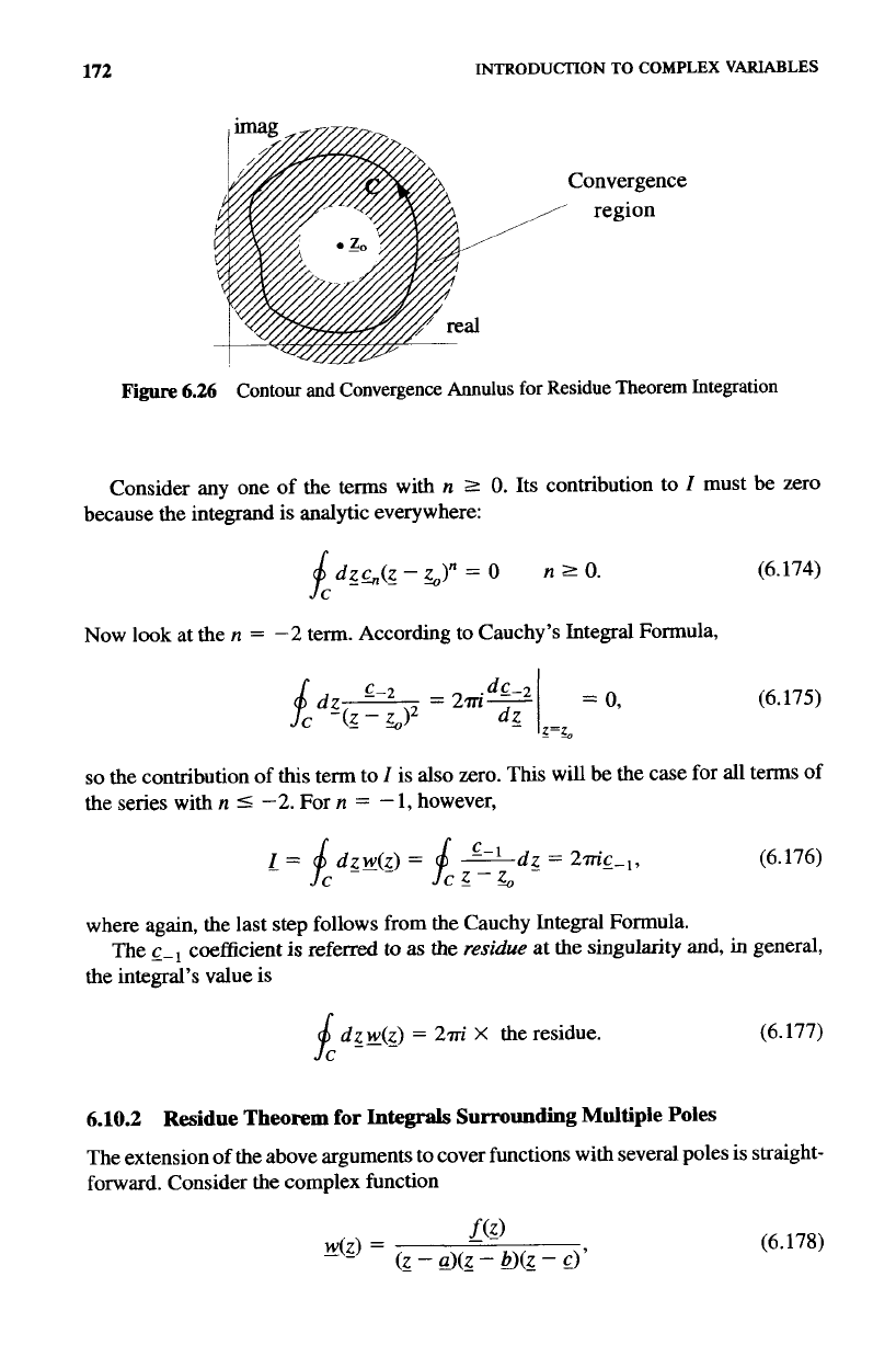
Figure 6.27
The Residue Theorem Applied
to
Multipoled
Functions
where
f(z)
is analytic in the entire g-plane. There are three poles at
z
=
a,
z
-
=
b,
and
g
=
c.
Imagine we are interested in evaluating
an
integral
L
=
idzw(&
(6.179)
where
C
encloses two
of
the poles of
~(z),
as
shown in Figure
6.27.
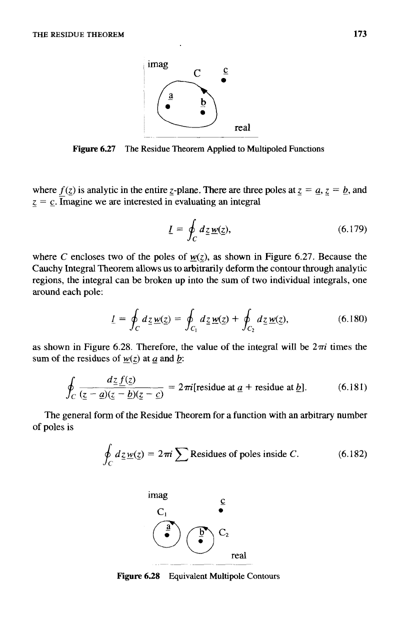
Because the
Cauchy Integral Theorem allows us to arbitrarily deform the contour through analytic
regions, the integral can be broken up into the sum of two individual integrals, one
around each pole:
(6.180)
as shown in Figure
6.28.
Therefore, the value of the integral will be
2m'
times the
sum
of
the residues
of
~(z)
at
g
and
b:
=
2m"residue at
Q
+
residue at
b].
(6.18
1)
d
z
f(z>
.f
c
(z
-
a&
-
b)(z
-
c)
The general
form
of
the Residue Theorem for
a
function with
an
arbitrary number
of
poles is
dzy(z)
=
27ri
Residues of poles inside
C.
(6.182)
(7
8"
real
~-
~~-
Figure 6.28
Equivalent
Multipole
Contours
174 INTRODUCTION TO
COMPLEX
VARIABLES
6.10.3
Residue
Formulae
Now that we have shown why residues are important, we need to develop some
methods for calculating them. We showed earlier that the residue
of
a singularity is
just the
c-,
term in a Laurent series expanded around the singularity itself. Thus, we
can always determine the residue
of
a singularity once we know the Laurent series.
Sometimes
this
is the only way possible, but in many cases we don’t have to do that
much work.
Imagine
we
already know that
a
singularity at
g
=
11
is
a first-order pole. The
Laurent series for such
a
pole, expanded about the pole, looks like
this,
(6.183)
c-
1
w(z)
=
-
+
5
+
Cl(Z
-
UJ
+
&
-
d2
+
*.‘,
(z
-
d
-
with no terms for
n
<
-
1.
Multiplying
this
series by
(z
-
UJ
gives
(6.184)
3
-_
w(z)(z
-
-
UJ
=
c-1
+
&(g
-
UJ
+
cl(z
-
UJ2
+
c&
-
4
+
*
* *
.
If
then
we
take the limit as
z
--+
11,
we find that
limk(&
-
41
=
c-1.
(6.185)
z-+g
This
gives a very simple method for determining the residue
of
a first-order pole.
As
an
example, consider the function
(6.186)
which has first-order poles at both
z
=
z
=
g:
and
z
=
b.
Let’s calculate the residue at
-
(6.187)
sing
(2-UJ
=-
1
(g-bJ.
limb(&
-
a)]
=
lim
z-n
This
method can be extended
for
the residues
of
higher-order poles. The Laurent
expansion
of
a second-order pole located at
z
=
a,
expanded around the pole, has the
form
(6.188)
Multiplication by
(Z
-
d2
gives
Now
we take the derivative
(6.190)
DEFINITE INTEGRALS AND CLOSURE
175
and finally take the limit as
z
+
a:
(6.191)
This gives
us
a simple formula for calculating the residue of a second-order pole. For
a pole
of
order
n
located at
z
=
a,
Equation 6.191 generalizes to
(6.192)
6.11
DEFINITE
INTEGRALS
AND
CLOSURE
The residue theorem can be used to evaluate certain types of real, definite integrals
which appear frequently in physics and engineering problems. The method involves
converting a real integral into a complex contour integral and then
closing
the con-
tour. The residue theorem can then
be
used
to evaluate the contour integral, and
subsequently the original definite integral.
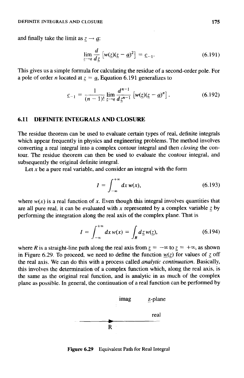
Let
x
be a pure real variable, and consider an integral with the form
(6.193)
where
w(x)
is a real function
of
x.
Even though
this
integral involves quantities that
are all pure real, it can be evaluated with
x
represented by a complex variable
2
by
performing the integration along the real axis
of
the complex plane. That
is
dx
w(x)
=
/
dg w@,
(6.194)
where
R
is
a straight-line path along the real axis from
z
=
--oo
to
z
=
+m,
as shown
in Figure 6.29. To proceed, we need to define the function
w(g)
for values of
z
off
the real axis. We can do this with a process called
analytic
continuation.
Basically,
this involves the determination
of
a complex function which, along the real axis,
is
the same as the original real function, and is analytic in as much of the complex
plane as possible. In general, the continuation of a real function can be performed by
z=1;
R
imag
-
z-plane
real
L
-
R
Figure
6.29
Equivalent Path
for
Real Integral