Kusse B.R., Westwig E.A. Mathematical Physics: Applied Mathematics for Scientists and Engineers
Подождите немного. Документ загружается.

236
FOURIER SERIES
question now is, does the sum over
k
in
Equation
7.65
lead to
an
orthogonality
condition that allows a determination of the
~'s
in Equation
7.64?
Answering
this
question will take some work.
Equation
7.65
can
be
rewritten
as
2N-1
Ur-1
(7.66)
k=O
k=O
where we have substituted
on
=
2m/T0.
Defining
eiR(n-m)
(7.67)
the sum in the
RHS
of
Equation
7.66
can
be
recognized as a geometric series, which
can
be
expressed
in
closed form
as
1
-IUr
1-r
2N-1
Crk==.
k=O
The summation
in
Equation
7.66
can therefore be written
as
(7.68)
(7.69)
Because
n
and
m
are both integers, the numerator of Equation
7.69
is
always
zero.
The
LHS
of
this
equation is therefore zero unless the denominator is
also
zero.
This
occurs when
n
-m
=
0,+2N,24N
,....
(7.70)
From our original definition, the integers
n
and
m
range from
zero
to the unspecified
limit
n,,
of
the sum
in
Equation
7.64:
(7.71)
If
we limit the sum
in
Equation
7.64
to
UV
terms, that is
n,,
=
2N
-
1,
we can force
In
-
ml
5
2N
-
1.
(7.72)
This
important result makes the denominator
of
Equation
7.69
zero
only
when
n
=
m.
This
is
exactly what we
need
to
construct the
orthogonality
condition.
All
that remains
is to evaluate Equation
7.69
for
n
=
m.
We can easily accomplish
this
by returning
to
Equation
7.66
and
substituting
(n
-
m)
=
0.
Our
final
orthogonality
condition
becomes
2h-
1
(7.73)
237
THE DISCRETE FOURIER SERIES
This
orthogonality condition can now
be
used to invert Equation
7.64
and eval-
uate
the
c,
for the discrete Fourier series.
To
do
this,
we multiply both sides
of
Equation 7.64 by
e-''+Jk
and sum over
k:
2N-1 2N-
1
m-
I
k=O
k=O
n=O
ur-1
ur-1
Using the orthogonality condition gives
2N-
1
2N-1
e-iomgfk
=
~,6,,,,,2N,
(7.74)
k=O
n=O
with the result that
(7.75)
Thus the original equation pair which defines the Fourier series can, for the discrete
Fourier series, be replaced by:
m
2N-
1
(7.76)
n=-m
n=O
7.4.2
Matrix
Formulation
Equations 7.76 and 7.77 are easily converted to a matrix format, which in turn,
is
easily handled by a computer. If we define the elements
of
the matrix
[MI
as
(7.78)
M~~
=
eimnrk
=
ei$nk
Equation 7.76 can be written using subscript notation as
fk
=
GMlk.
Likewise, Equation 7.77 becomes
(7.79)
1
Cn
-
-MLfk.
2N
-
(7.80)
FOURIER
SERIES
238
The orthogonality condition, Equation 7.73, is simply
M&ML
=
6,,,,,2N.
(7.81)
Keep
in
mind, the subscripts of
all
these expressions
run
from
0
to
2N
-
1.
Notice that the
[MI
ma&
is
the same for
all
functions, it
only
depends upon the
number of sample
points.
The computer obtains the coefficients of the discrete Fourier
series by inserting the sampled values of
f(t)
into Equation
7.80
and performing the
summations.
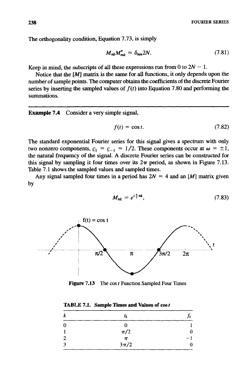
Example
7.4
Consider a very simple signal,
f(t)
=
cost. (7.82)
The standard exponential Fourier series for
this
signal gives
a
spectrum with
only
two
nonzero components,
c1
=
_c-
I
=
1
/2.
These components occur at
w
=
&
1,
the natural frequency
of
the signal.
A
discrete Fourier series can
be
constructed for
this
signal by sampling it four times over its
2m
period,
as
shown in Figure 7.13.
Table 7.1
shows
the sampled values and sampled times.
Any signal sampled
four
times
in
a period has
W
=
4
and an
[MI
matrix given
by
Mnk
=
(7.83)
I
f(t)
=cost
I
I
,
I
8
I
I
I
-
____
I
Figure
7.13
The
cos
I
Function
Sampled
Four Times
TABLE
7.1.
Sample
Times
and
Values
of
cost
k
tk
.h
0
.rr/2
7r
3
1r/2
1
0
-1
0
THE
DISCRETE
FOURIER
SERIES
239
which in matrix array notation
is
Using Equation
7.80,
we can evaluate the
c,,
11
with the result that
(7.84)
(7.85)
(7.86)
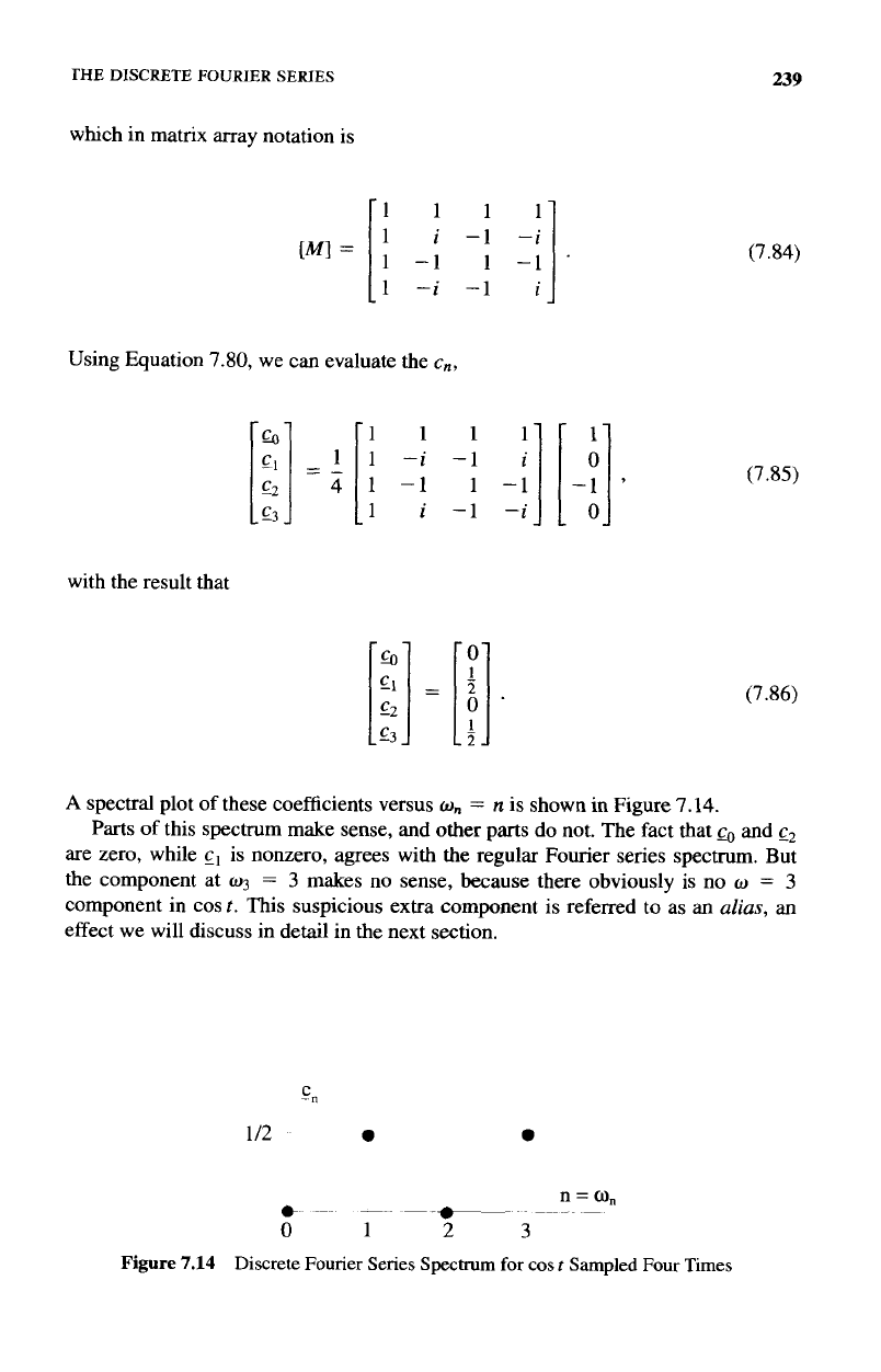
A
spectral plot
of
these coefficients versus
w,
=
n
is shown in Figure
7.14.
Parts
of this spectrum make sense, and other parts do not. The fact that and
c,
are zero, while
c1
is nonzero, agrees with the regular Fourier series spectrum. But
the component at
03
=
3
makes no sense, because there obviously is no
w
=
3
component in
cos
t.
This suspicious extra component is referred to as an
alias,
an
effect
we
will discuss in detail in the next
section.
-cn
1
I2
0 0
n
=
on
*-
-
-.--
~
0
1
2
3
Figure
7.14
Discrete Fourier Senes
Specbum
for
cos
t
Sampled
Four
Times
240
FOURIER
SERIES
Now let’s see how the coefficients give us back the sampled values of the function.
Equation
7.79
written for
this
example becomes
(7.87)
n=O
n=O
Inserting the values for
&
and noting that
tk
=
kTo/(2N)
=
kv/2,
The
RHS
of Equation
7.88
sums
to the proper, real value of cos
t
at
the
sample times
t
=
0,
v/2
,
m,
and
3v/2.
At other vdues oft
#
tk,
the
ms
of Equation
7.88
does
not equal
f(t)
and
is
not even pure real! In order for Equation
7.76
to be a good
representation of the original
f(t),
it seems we must sample the signal many times.
We will quantify
this
statement in the following sections and in the next chapter.
7.4.3
Aliasing
In
the previous section,
the
discrete Fourier series technique was applied to the
function
f(t)
=
cos
t
and it was sampled four times. The resulting spectrum, shown
in Figure
7.14,
had a legitimate component at
w
=
1
and an erroneous one at
w
=
3.
We
called the
w
=
3
component an alias. What is the source of
this
alias, and what
parts of a discrete spectrum are to be trusted?
The alias arises from the simple fact that when four sampling points are used,
the
two functions cos
t
and cos
3t
give exactly the same values at the sampling points
(0,
v/2,
v.
3v/2,2~).
We can remove the alias at
w
=
3
by sampling more times per
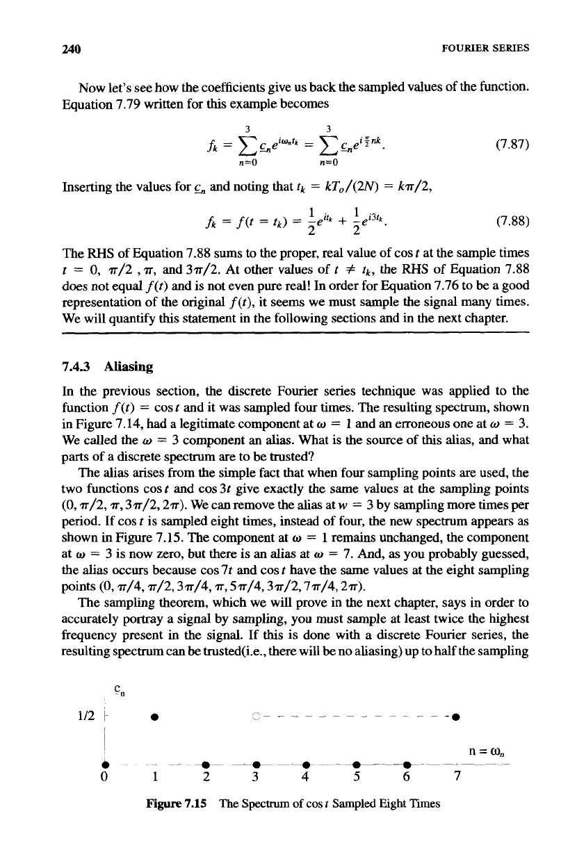
period. If cos
t
is sampled eight times, instead of four, the new spectrum appears
as
shown in Figure
7.15.
The component at
w
=
1
remains unchanged, the component
at
w
=
3
is
now zero, but there
is
an
alias
at
w
=
7.
And, as you probably guessed,
the alias occurs because cos
7t
and cos
t
have the same values at the eight sampling
points
(0,
v/4, v/2,3~/4,
T,
5~/4,3~/2,7~/4,2~).
The sampling theorem, which we will prove in the next chapter, says in order
to
accurately portray a signal by sampling, you must sample at least twice
the
highest
frequency present in the signal. If
this
is
done with a discrete Fourier series, the
resulting spectrum can be trusted(i.e., there will
be
no aliasing) up to half the sampling
cn
Figure
7.15
The
Spectrum
of
cos
t
Sampled
Eight
Times
241
THE
DISCRETE FOURIER SERIES
frequency. Therefore, the spectrum of Figure 7.14 is valid up to
n
=
on
=
2,
while
the spectrum of Figure 7.15 is valid up to
n
=
on
=
4. The signal
fit)
=
cos
f
+
cos 3t
(7.89)
has a period
T,,
=
2~r
and must be sampled at a frequency of 6, or six times over that
interval, in order to trust the sampled spectrum up
to
n
=
on
=
3.
7.4.4
Positive and Negative Frequencies
The normal exponential Fourier series contains terms for both positive and negative
frequencies. The discrete Fourier series, the way it was developed in the discussion
above, created a spectrum that ranged
in
n
from
0
to
(2N
-
1)
or
0
5
on
5
27~(2N
-
l)/To.
To
establish this orthogonality condition of Equation 7.73, however,
it is only necessary that
n
take on
2N
consecutive values. The discrete series analysis
can therefore be set
up
with all the
sums
over
n
starting at some arbitrary integer, say
no,
and ranging to
(2N
+
no
-
1) where
2N
is
still the number of sampled points in
the period. Equation 7.76, for example, could have been written as
2N+n,-1
(7.90)
n=no
The elements
of
the
[MI
matrix are generated by the same set of
k
values, but a shifted
set of
n
values:
(7.91)
Except for these modifications, the development of the discrete Fourier series would
be unchanged.
This flexibility in selecting the value of
no,
coupled with the sampling theorem,
allow discrete Fourier series spectra to be set up more like the regular exponential
Fourier spectra. If we set
no
to
-N,
then the sums over
n
range from
-N
to
(N
-
1)
and the spectra that result will range in frequency from
-2.rrN/TO
to
27iN
-
1)/To.
If, in addition, the signal is sampled at a rate
of
at least twice the highest frequency
present, there will be no aliasing in the spectrum that results
from
the discrete Fourier
series analysis.
Taking
such a range
for
n,
the two spectra shown in Figures 7.14 and
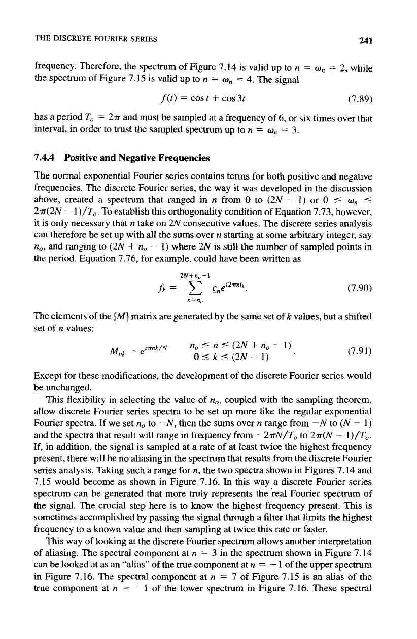
7.15 would become
as
shown in Figure 7.16. In this way a discrete Fourier series
spectrum can be generated that more truly represents the real Fourier spectrum of
the signal. The crucial step here is to know the highest frequency present.
This
is
sometimes accomplished by passing the
signal
through a filter that limits the hghest
frequency to a known value and then sampling at twice this rate or faster.
This way of looking at the discrete Fourier spectrum allows another interpretation
of aliasing. The spectral component at
n
=
3
in the spectrum shown in Figure 7.14
can be looked at as an “alias” of the true component at
n
=
-
1
of the upper spectrum
in Figure 7.16. The spectral component at
n
=
7
of
Figure 7.15 is
an
alias
of
the
true component at
n
=
-
1
of
the lower spectrum in Figure 7.16. These spectral
242
FOURIER
SERIES
[
-c.
0
112
c
0
N=2
n=w,
I
+-
L.,
-2
-1
0
1
,
-Cn
0
112
1
0
N=4
I
n=o,
I
I
*
1
a
w
I
c
w
-4
-3
-2
-1
1 2
3
Figure
7.16
The Discrete Fourier Series
Spectrum
for
-N
S
n
5
(N
-
1)
components are being moved around by the shifting that occurs in the
[MI
matrix as
no
is
changed, as described by Equation 7.91.
Notice that with the
almost
symmetric choice for the range
of
n
demonstrated by
the
spectra
in Figure 7.16, the discrete Fourier
Series
representation for the sampled
values
of
cos
t
becomes
N-
1
n=-N
(7.92)
The
RHS
of Equation 7.92
is
not only pure real and equal to cost at the sampled
values,
t
=
tk, but
is
also
pure real and eqd
to
cos
t
for values
of
t
!
EXERCISES
FOR
CHAPTER
7
1.
Show that
if
f(t)
is
a periodic function with period
To,
then
f(t>
=
f(t
+
3Td.
A
Fourier series
for
f(t)
can be constructed that uses
wn
=
2m/3T0. Show that
this is the same Fourier series that
is
generated using
w,
=
2nn/T0.
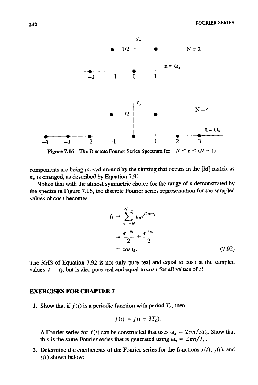
2.
Determine the coefficients of the Fourier series for the functions
x(t),
y(t),
and
z(t)
shown below:
EXERCISES
243
2
3.
Consider the exponential Fourier series for
f(x)
with the form
n=-m
Answer the following questions without actually determining the Fourier coeffi-
cients:
(a)
If
f(x)
=
sin2
x,
what are the values for the
on?
(b)
If
f(x)
=
sin2
x,
is
Q,
zero or nonzero?
(c)
If
f(x)
=
sin2
x,
are the
c,
pure red, pure imaginary, or complex?
(d)
If
f(x)
=
sin2
(x
-
7r/2),
are the pure real, pure imaginary, or complex?
(e)
If
f(x)
=
sin2
(x
-
7r/4),
are the pure real, pure imaginary, or complex?
Now determine
all
the exponential Fourier series coefficients for
f(x)
=
sin2
x,
without doing any integrals.
4.
Determine the sinekosine Fourier series that represents the following periodic
function:
FOURIER
SERIES
244
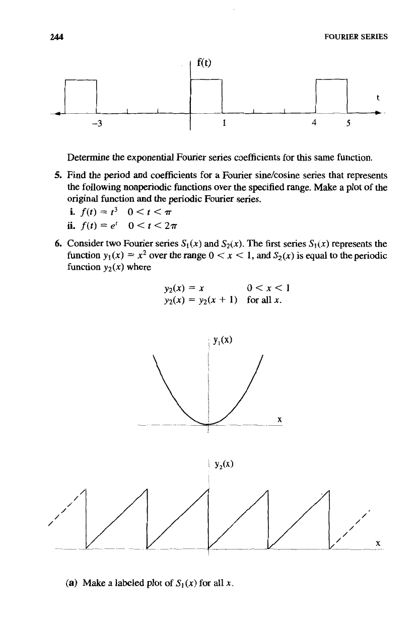
1
4
5
-3
I
Determine
the exponential Fourier series coefficients for
this
same function.
5.
Find the period and coefficients for a Fourier sinekosine series that represents
the following nonperiodic functions over the specified range. Make a plot of the
original function and
the
periodic Fourier series.
i.
f(t)
=
t3
o
<
t
<
T
ii.
f(t)
=
et
0
<
t
<
2~
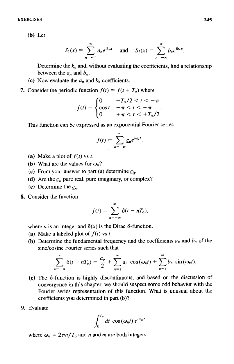
6.
Consider two Fourier series
Sl(x)
and
S2(x).
The
first series
Sl(x)
represents the
function
yl(x)
=
x2
over the range
0
<
x
<
1,
and
&(x)
is
equal to the periodic
function
y2(x)
where
YZ(X)
=
x
O<x<l
y2(x)
=
y2(x
+
1)
for all
x.
(a)
Make
a
labeled plot of
S1
(x)
for all
x.
EXERCISES
245
(b)
Let
nc
m
s~(x)
=
C
aneiknx
and
&(x)
=
bneiknx.
Determine the
k,
and, without evaluating the coefficients, find a relationship
between the
a,
and
b,.
(c)
Now
evaluate the
a,
and
b,
coefficients.
7.
Consider the periodic function
f(t)
=
f(t
+
To)
where
0
-T0/2<t<
-IT
f(t)
=
cost
-n<t<
+7r
.
{
0
+Tr<t<
+T0/2
This function can
be
expressed
as
an exponential Fourier series
n=--pl
(a)
Make a plot
of
f(t)
vs
t.
(b)
What are the values for
w,?
(c)
From your answer to
part
(a) determine
G.
(d)
Are the
c,
pure real, pure imaginary, or complex?
(e)
Determine the
cn.
8.
Consider the function
m
f(t)
=
c
-
nToh
n=-m
where
n
is an integer and
6(x)
is the Dirac &function.
Make a labeled plot
of
f(t)
vs
t.
Determine the fundamental frequency and the coefficients
a,
and
b,
of
the
sinelcosine Fourier series such that
1
m
cc
8(t
-
nTo)
=
7
+
an
cos
(w,t)
+
b,
sin
(w,t).
n=l
1
n=-s
n=I
The &function is highly discontinuous, and based on the discussion of
convergence in this chapter, we should suspect some odd behavior with the
Fourier series representation of
this
function. What is unusual about the
coefficients you determined in
part
(b)?
9.
Evaluate
1"
dt
cos
(w,t)
eiam',
where
w,
=
2nn/T0
and
n
and
m
are both integers.