Kusse B.R., Westwig E.A. Mathematical Physics: Applied Mathematics for Scientists and Engineers
Подождите немного. Документ загружается.

316
LAPLACE
TRANSFORMS
Figure
9.13
The
Heaviside Step Function
This
final result comes from the orthogonality relation derived
in
the previous chapter.
Equation
9.37
is
actually a more general form of that orthogonality relation:
(9.39)
9.4.2
The
Heaviside
Function
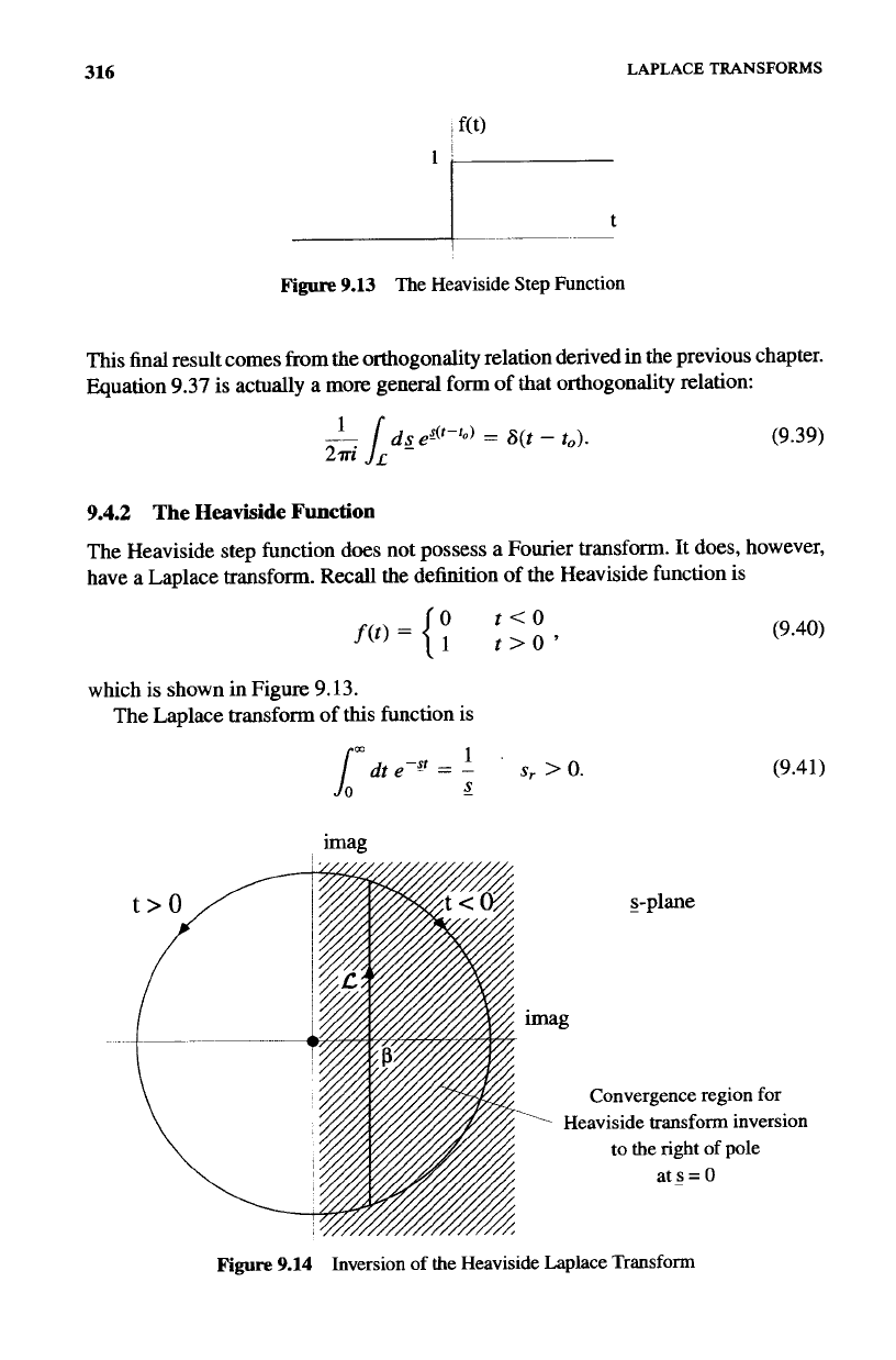
The Heaviside step function does not possess a Fourier transform. It does, however,
have a Laplace transform.
Recall
the definition of the Heaviside function is
which
is
shown in Figure 9.13.
The Laplace transform
of
this
function is
(9.40)
(9.41)
imag
s-plane
imag
Convergence region
for
Heaviside
transform
inversion
to
the
right
of
pole
ats=O
Figure
9.14
Inversion
of
the
Heaviside
Laplace
Transform
LAPLACE TRANSFORM EXAMPLES
317
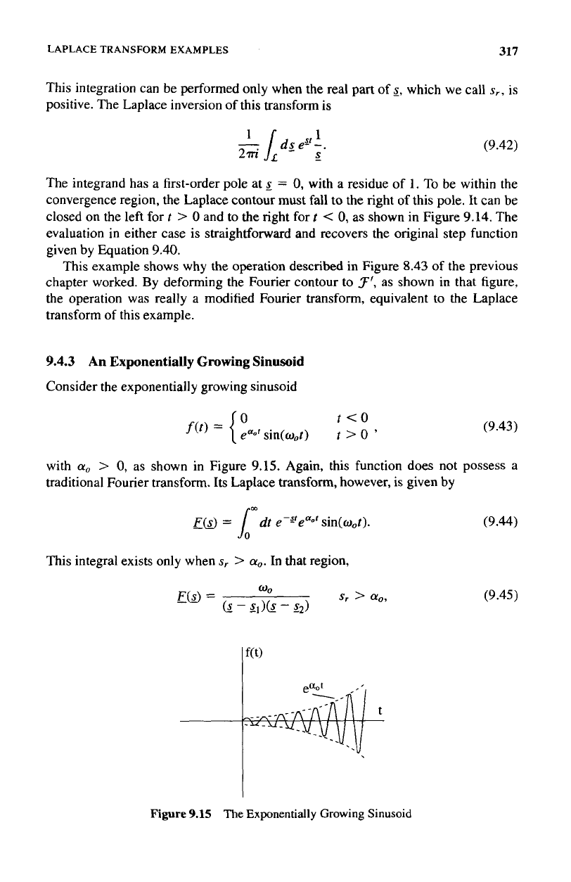
This integration can be performed only when the real part of
3,
which we call
s,,
is
positive. The Laplace inversion of this transform is
(9.42)
The integrand has a first-order pole at
5
=
0,
with a residue
of
1.
To be within the
convergence region, the Laplace contour must fall to the right of this pole. It can be
closed
on
the left for
t
>
0
and to the right for
I
<
0,
as shown
in
Figure 9.14. The
evaluation
in
either case is straightforward and recovers the original step function
given by Equation 9.40.
This example shows why
the
operation described in Figure 8.43
of
the previous
chapter worked.
By
deforming the Fourier contour
to
F‘,
as shown in that figure,
the operation was really a modified Fourier transform, equivalent to the Laplace
transform
of
this example.
9.4.3
An
Exponentially
Growing
Sinusoid
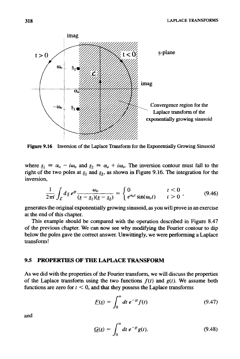
Consider the exponentially growing sinusoid
(9.43)
with
a,
>
0,
as shown in Figure 9.15. Again, this function does not possess a
traditional Fourier transform. Its Laplace transform, however, is given by
E(s>
=
Lrn
dt
e-sfeael
sin(o,t).
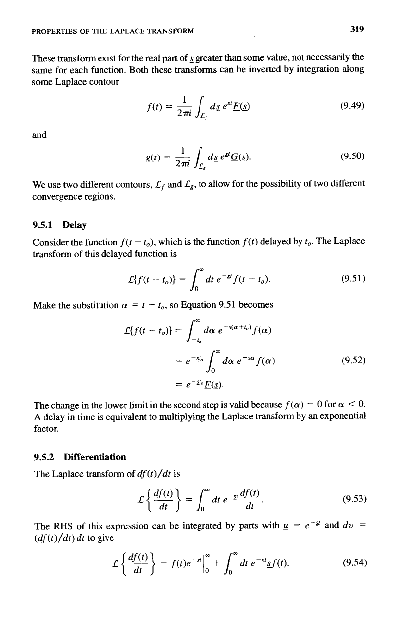
This integral exists only when
s,
>
a,.
In
that region,
(9.44)
(9.45)
Figure
9.15
The
Exponentially Growing
Sinusoid
318
imag
imag
LAPLACE
TRANSFORMS
s-plane
Convergence region
for
the
Laplace
transform
of
the
exponentially growing sinusoid
1
Figure
9.16
Inversion
of
the Laplace
Transform
for
the
Exponentially
Growing
Sinusoid
where
s,
=
a,
-
io,
and
s2
3
a,
+
io,.
The inversion contour must fall to the
right of the two poles at
g,
and
g2,
as
shown in Figure 9.16. The integration for the
inversion,
generates the original exponentially growing sinusoid,
as
you
will prove in
an
exercise
at the end
of
this
chapter.
This
example should
be
compared with the operation described in Figure 8.47
of
the previous chapter. We can now
see
why modifying the Fourier contour to dip
below the poles gave the correct answer. Unwittingly, we were performing a Laplace
transform!
9.5
PROPERTIES OF THE LAPLACE TRANSFORM
As
we did with the properties of the Fourier transform, we will discuss the properties
of the Laplace transform using the two functions
f(t)
and
g(t).
We assume both
functions are zero for
t
<
0,
and that they possess the Laplace transforms
and
(9.47)
G(s)
=
1
dt
e-”g(t).
(9.48)
PROPERTIES
OF
THE LAPLACE TRANSFORM
319
These transform exist for the real part of
s
greater than some value, not necessarily the
same for each function. Both these transforms can be inverted by integration along
some Laplace contour
and
(9.49)
(9.50)
We use two different contours,
Lf
and
L,,
to allow for the possibility of two different
convergence regions.
9.5.1
Delay
Consider the function
f(t
-
to),
which is the function
f(t)
delayed by
to.
The Laplace
transform of this delayed function is
m
L{f(t
-
to)}
=
A
dt
e-xt
f(t
-
to).
Make the substitution
a
=
t
-
to,
so
Equation 9.51 becomes
L{f(t
-
to)}
=
[:o
da
e-s(u+'o)
f(a)
(9.5
1)
(9.52)
The change in the lower limit in the second step is valid because
f(a)
=
0
for
a
<
0.
A
delay in time is equivalent to multiplying the Laplace transform by an exponential
factor.
9.5.2
Differentiation
The Laplace transform
of
df(t)/dt
is
(9.53)
The
RHS
of this expression can be integrated by parts with
g
=
e-3'
and
dv
=
(df(t
j/dt
j
dt
to
give
(9.54)
320
LAPLACE TRANSFORMS
If the real part of
.r
is large enough to make
f(t)e-s'
go to zero as
t
--+
m,
then
L{Y}
=
-f(O)+gE(sJ.
(9.55)
Notice the difference between
this
result and the derivative relationship for the Fourier
transform.
9.5.3
Convolution
Now consider a function
h(t),
which is the convolution of
f(t)
with
g(t):
h(t)
=
dr f(r)g(t
-
7).
L
(9.56)
The Laplace transform of
h(t)
can be written as
rm
=
1:
dt ePSth(t)
=
1:
dt e-s'
1:
dr
f
(r)g(t
-
7).
(9.57)
In the second step, we extended the lower limit to
-m
using the result of Exercise 8.15,
which says if
f(t)
=
0
and
g(t)
=
0
for
t
<
0,
then
h(t)
=
0
for
t
<
0.
Now
substitute the inverse Laplace transforms for
f(~)
and
g(t
-
T)
to convert the
RHS
of
Equation 9.57 into
f
(7)
g(f--7)
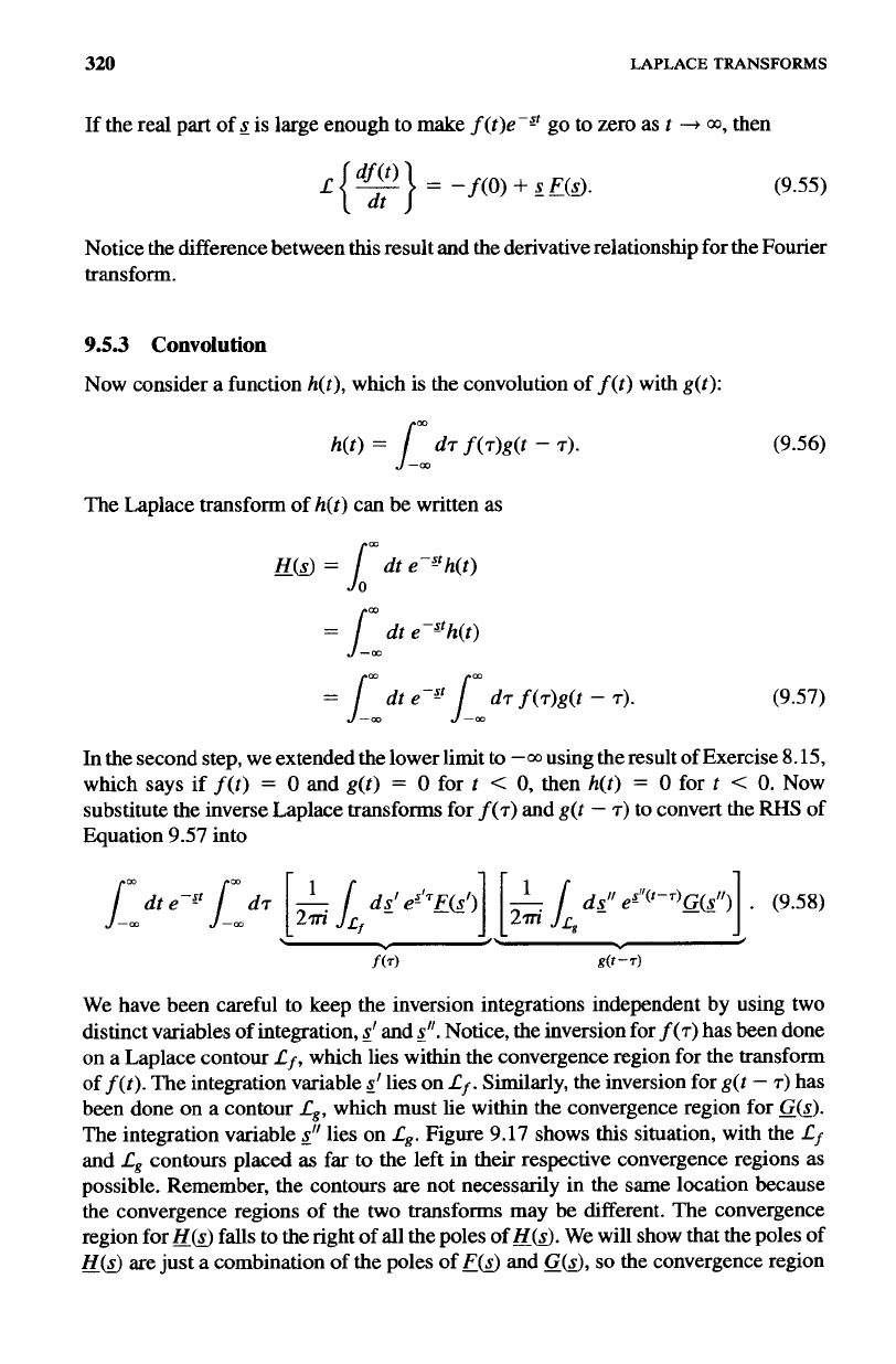
We have been careful to keep the inversion integrations independent by using two
distinct variables of integration,
g'
and
s".
Notice, the inversion for
f(
T)
has been done
on a Laplace contour
Lf,
which lies within the convergence region for the transform
of
f(t).
The integration variable
s'
lies on
Lf.
Similarly, the inversion for
g(t
-
r)
has
been done on a contour
L,,
which must lie within the convergence region for
G(s).
The integration variable
5''
lies on
L,.
Figure 9.17 shows this situation, with the
Lf
and
L,
contours placed
as
far to the left in their respective convergence regions as
possible. Remember, the contours are not necessarily in the same location because
the convergence regions of the
two
transforms may be different. The convergence
region for
230
falls to the right of all the poles of
IYW.
We will show that the poles
of
g(s>
are just a combination of the poles of
&YJ
and
GO,
so
the convergence region
PROPERTIES
OF
THE LAPLACE TRANSFORM
321
Convergence region
for
transform of
f(t)
.-
imag
I
s-plane
c
Convergence region
for transform
of
g(t)
Figure
9.17
Convergence Regions
and
Laplace Contours
for
f(t)
and
g(t)
of
li[(s)
is just the overlap
of
the convergence regions of
E(s)
and
c(s).
The variable
Because
L,
is to the right of
all
the poles
of
EsJ,
and
.L,
is to the right of all the
poles of
G(s),
contour deformation allows
us
to move both
.Lf
and
Lg
to the right
without changing the values of their integrals. It will be very convenient if we move
them to the right
so
that they become a common contour
L
that passes through the
point
s.
Remember
s
is
the point where we want to evaluate
HsJ.
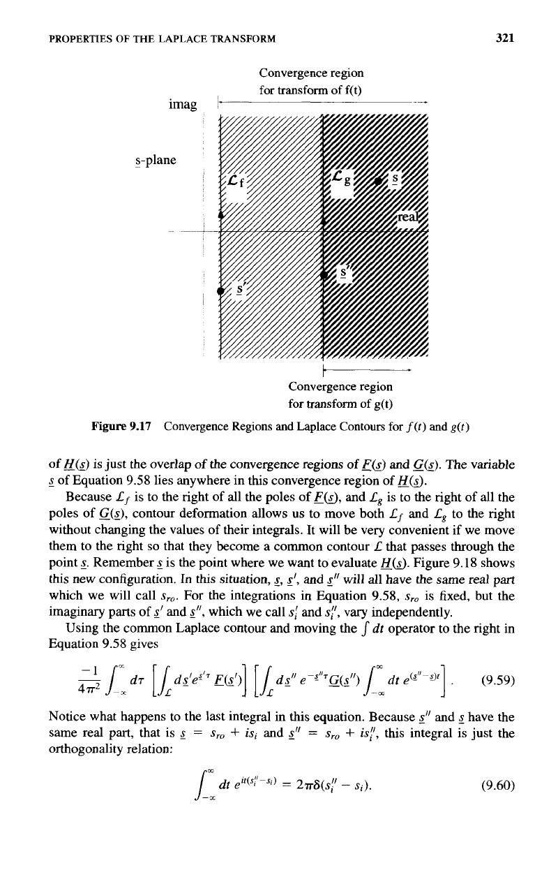
Figure 9.18 shows
this new configuration.
In
this situation,
g,
s‘,
and
$‘
will all have the same real
part
which we will call
s,.
For the integrations in Equation 9.58,
sro
is fixed, but the
imaginary parts
of
8’
and
s”,
which we call
s:
and
s:,
vary
independently.
dt
operator to the right in
Equation 9.58 gives
of Equation 9.58 lies anywhere in this convergence region of
@(sJ.
Using the common Laplace contour and moving the
Notice what happens to the last integral in this equation. Because
s”
and
s
have the
same real
part,
that is
=
s,
+
is,
and
s’’
=
s,
+
is:,
this integral is
just
the
orthogonality relation:
[I
dt
ert(s:-sc)
=
2
7rS(S:’
-
s,).
(9.60)
322
LAPLACE
TRANSFORMS
s-plane
j
-7
I
Figure
9.18
The Common Region
of
Convergence
and
Laplace Contour
Applying
this
to expression 9.59 gives
where we have also made use of the fact that along
L,
ds“
=
ids;,
with
s:
ranging
from minus to plus
infinity.
The 8-function makes
the
integral over
s“
very easy and
lets us write
Interchange the remaining two integrals:
(9.62)
(9.63)
We can now pull a similar stunt
to
the one used on the last integral in Equation 9.59.
Because
2’
and
3
have the same real part,
this
looks like another instance
of
the
orthogonality relation:
J_mm
dr
ei7(s:-sJ)
=
2T8(Sl
-
Si).
(9.64)
Again making use
of
the fact that
ds’
=
ids;
along the
L
contour, we can write
=
-
F(S)GsJ.
(9.66)
PROPERTIES
OF
THE LAPLACE TRANSFORM
323
This is an elegant final result. The Laplace transform of the convolution
of
two
functions is the product of the Laplace transforms of the functions
Because
H(s)
is the product of
F(s)
and
GO,
the poles of
H(s)
are just a combination
of the poles
of
and
G(s).
The convergence region for
H(sJ
is therefore the
intersection
of
the convergence regions
of
both
E(s)
and
GO,
as we assumed earlier.
9.5.4
Multiplication
As a final situation, consider the product of two functions
The Laplace transform
of
h(t)
is given by
rm
H(S)
=
dt
e-”’f(t)g(t)
(9.68)
(9.69)
Again
f(t)
and
g(t)
have been assumed to be zero for
t
<
0,
so
that the
dt
integration
of the Laplace transform can
be
extended to negative
infiNty.
As
with the previous
case, the Laplace contours
Lf
and
L,
are in their respective convergence regions and,
initially, are placed as far to the left as possible, as shown in Figures 9.17 and 9.19.
We begin the manipulation of Equation
9.69
by interchanging the order of inte-
gration, to obtain:
On
Lf
let
$
=
s:,
+
is;
and on
L,
let
5’’
=
If
s
=
s,
+
isi,
then in order for the
dt
integral to exist, we must have
+
is:
where
s:,
and
s;;
are constants.
s;,
+
s;,
-
s,
=
0.
(9.71)
If the condition is not met, the
dt
integral diverges and
I%($
does not exist.
If
this
condition is met, however, the
dt
integral becomes a 8-function,
(9.72)
=
2rtqs;
+
s:
-
Si),
(9.73)
and
H(s)
can be evaluated.
The condition of Equation 9.71 constrains the convergence region of
H(s).
If
F($)
converges for
si
>
sf
and
G(g”)
converges for
s:
>
sg,
then Equation 9.71 says
H(sJ
can exist only for
s,
>
sf
+
sg.
This
situation is shown in Figure
9.19.
To see why
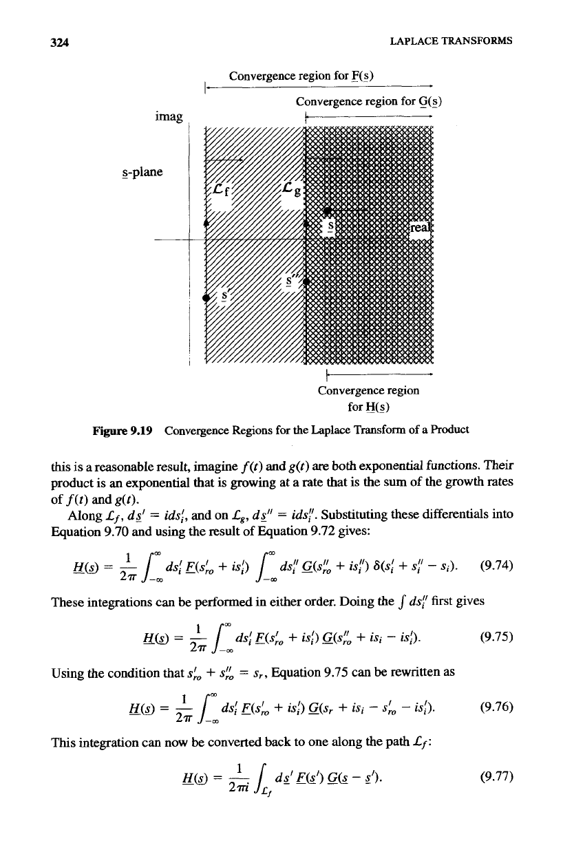
324
Convergence region for
F(s)
LAPLACE TRANSFORMS
I--
~
Convergence region for
G(s)
imag
~
s-plane
-
t
Convergence region
for
HW
Figure
9.19
Convergence Regions for the Laplace Transform of a Product
this
is a reasonable result, imagine
f(r)
and
g(t)
are
both exponentid functions. Their
product is
an
exponential that
is
growing at
a
rate that
is
the sum of the growth rates
Along
Lf,
dz'
=
idsf,
and on
Lg,
d$'
=
ids:.
Substituting these differentials into
of
f(0
and
g(0.
Equation
9.70
and using the result of Equation
9.72
gives:
m
m
H(S)
-
=
1
ds;
E(si,
+
is;)
ds:
G(s:o
+
is:)
S(si
+
s;
-
si).
(9.74)
2T
--m
These integrations
can
be performed in either order. Doing the
dsf'
first gives
HSJ
=
-
ds;
~(s:,
+
is;)
~(s:,
+
isi
-
is;).
(9.75)
2m
Sm
-m
Using the condition that
s:,
+
s:,
=
sr,
Equation
9.75
can
be
rewritten as
This integration can now be converted back
to
one along the path
Lf:
(9.77)
PROPERTIES
OF
THE LAPLACE TRANSFORM
325
Notice the result of Equation 9.77 is similar to the convolution integral discussed
earlier, except now the integration
is
done along a complex path. The result
of
Equation 9.77 can be written in a shorthand notation as
If the order of the integration of Equation 9.74 is reversed the result becomes
(9.78)
(9.79)
We
have obtained a result that is similar to the one for Fourier transforms. The
Laplace transform of the product of
two
functions
is
the convolution of the separate
transforms. In this case, however, the convolution must be integrated on one of the
Laplace contours.
In arriving at Equation 9.77
s,
was determined by the locations of the
Lf
and
Lg
contours according to the condition
s,
=
s:,
+
s:~.
As
the
Lf
and
L,
contours are
moved to
the
right,
S,
increases and consequently
8
also
moves to the right, as shown
in Figure 9.19. When using Equations 9.78 or 9.79 to evaluate
HsJ,
however, it is
convenient to take another point of view. In particular, when using Equation 9.77,
it makes more sense to select a fixed value for
g
and use
this
value to determine
the location of the
Lf
contour.
To
do this, it must be realized that only values of
s_
in the convergence region of
H(S)
can be used.
In
this
convergence region, all the
$-plane
poles
of
G(,r
-
g’)
must
be
to the right of
all
the $-plane poles of
&I).
This
condition can be used to define the convergence region for
fZsJ.
The integration of
Equation 9.77 is then evaluated by placing the
Lf
contour between the $-plane poles
of
E($)
and
G(s
-
s’).
These ideas are demonstrated in the following example.
Example
9.1
strated by a simple example. Let
The process
of
convolution
along
a Laplace contour can
be
demon-
and
The Laplace transforms of these functions are easily taken:
1
EN=-
5-2’
with a convergence region given by
s,
>
2,
and
(9.80)
(9.8
1)
(9.82)
(9.83)
1
GO=-
3-3’
-