Kusse B.R., Westwig E.A. Mathematical Physics: Applied Mathematics for Scientists and Engineers
Подождите немного. Документ загружается.

346
DIFFERENTIAL EQUATIONS
Notice, it must be possible to calculate the integral
of
P(x)
in order to use
this
method.
It is not necessary to worry about the constants of integration associated with the two
integrations performed in the steps above. The original differential equation we are
trying
to
solve
is
first
order, and therefore needs only one
arbitrary
constant.
This
constant will be introduced in the subsequent steps.
With
a(x)
determined, the solution to the original differential equation can now
be
obtained. Multiplying both sides
of
Equation 10.34 by
a(x)
and using Equation
10.35 gives
Integrating both
sides
results in the expression
a(x)y(x)
=
/dx
a(x)G(x)
+
C,.
(10.40)
The integration constant
C,
is determined by the single boundary condition that is
necessary to make the solution unique. The final result is
(10.41)
Notice that to use
this
process, not only must we be able to integrate the function
P(x)
to get
a(x),
but we must also be able to integrate the function
a(x)G(x).
Example
10.3
As
a simple example of using an integrating factor, consider the
differential equation
dY
-
+
y
=
ex,
dx
with the boundary condition y(0)
=
1. The integration factor is simply
a(x)
=
eJdx
=
ex.
Substitution into Equation 10.41 gives
(10.42)
(10.43)
(10.44)
1
2
=
-ex
+
Coe-x.
The
boundary condition requires
C,
=
1/2,
so
y(x)
=
cosh(x). (10.45)
TECHNIQUES FOR SECOND-ORDER EQUATIONS
347
10.3 TECHNIQUES FOR SECOND-ORDER EQUATIONS
Second-order differential equations pervade physics and engineering problems. One
of the most common equation in physics is the second-order equation
(10.46)
which describes the motion of a simple harmonic oscillator with a period of
2rr/w0.
As
mentioned earlier, the number of nontrivial, independent solutions of a linear
differential equation is equal to the order
of
the equation. Thus, a linear second-order
equation should have two different solutions. We can see that this is the case for
Equation 10.46, since both
y(x)
=
sin(o,x) (10.47)
y(x)
=
cos(wox) (10.48)
are valid solutions.
There is no general analytic method for finding solutions to second-order and
higher equations. Solutions are often obtained
by
educated guessing, or numerical
methods. There is a general technique, however, for a specialized class of equations
which have constant coefficients.
In
this
section, we describe a simple technique
for solving ordinary, second-order, linear differential equations with constant co-
efficients. Then we introduce an important quantity called the Wronskian, which
provides a powerful method for generating a second solution to
a
homogeneous dif-
ferential equation when one solution is known. The Wronskian can also help generate
the particular solution to a nonhomogeneous equation, if the general homogeneous
solution is already known.
10.3.1 Ordinary, Homogeneous Equations with Constant Coefficients
The most general form of a second-order, linear, ordinary, homogeneous differential
equation can be written as
d2yo
+
P(x)W
+
Q(x)
y(x)
=
0.
dx2 dx
(10.49)
Equation 10.49
is
said to have constant coefficients, if the functions
P(x)
and
Q(x)
are constants,
(10.50)
where the factor of
-
2
was used in the second term to simplify the algebra
to
come.
The manipulation of the linear equations
is
assisted by defining the differential
operator of order
n
as
D&
=
d"/dx".
In
this notation, Equation
10.50
becomes
348
DIFFERENTIAL EQUATIONS
We can now
perform
a fancy trick, and factor
this
as
if
it were
a
quadratic algebraic
expression,
(Dop
-
r+>(Dop
-
r-)y(x)
=
0,
(10.52)
-
where r2
=
p
2
dfi.
This
expression is completely equivalent to Equation
10.51.
This
can be solved in two
steps.
First solve for
s(x),
the bracketed term in Equation
10.52,
(10.53)
(Dop
-
r+)S(X)
=
0.
This
is a simple first-order equation with the solution
s(x)
=
Ae‘+’,
(
10.54)
where
A
is
our
first undetermined constant. The second step is to solve the remainder
of Equation 10.52:
(DOp
-
r-)y(x)
=
s(x)
=
Aer+x.
(10.55)
This
is another first-order equation. Its solution can
be
obtained by using
an
integration
factor of
e-r-x,
with the result
y(x)
=
er-x
B
+
A dxe
r+-r--)x
(10.56)
where we have left the integral indefinite and introduced
B,
our
second undetermined
constant.
At
this
point, there are two cases to consider. First, if
p2
=
4,
the two “roots” are
equal:
r-
=
r+
=
p.
In
this
case, Equation 10.56 becomes
y(x)
=
(Ax
+
B)ePX
forp2
=
4.
(10.57)
[
I(
1.
On the other hand,
if
p2
#
4,
then we get
y(x)
=
Ae‘+*
+
Be’-’
forp
#
4’.
(10.58)
In both cases, there are two arbitrary constants, which are determined by the boundary
conditions of the problem.
“What
if
the
roots
are
imaginary?” we hear you asking. In other words, what
happens if
p2
<
q,
forcing
r+
and r- to be complex? It
turns
out Equation 10.58
is still entirely valid,
if
you remember the complex definition of the exponential
function:
e(~+i~)
=
-
eX[cos
y
+
i
sin
y1.
(10.59)
If
p2
<
4,
r+
and
r-
will always
be
complex conjugates.
In
this
case, define
r-t
=
r,
2
iri
where r, is the real part of
r+,
and
ri
is the imaginary part of
r+ .
Using
this
definition and redefining the arbitrary constants converts Equation 10.58 into
y(x)
=
errx
[A
cos(rix)
+
B
sin(rix)]
for
p2
<
q.
(10.60)
TECHNIQUES FOR SECOND-ORDER EQUATIONS
349
Example
10.4
Consider the classic example of the harmonic oscillator, governed
by the second-order equation
(10.61)
In operator notation, this equation is represented by
Referring to Equation 10.50,
p
=
0
and
q
=
0,’.
The roots associated with
this
equation are
r-2
=
-+iw,.
When substituted into Equation 10.60,
the
general solution
for the simple harmonic oscillator becomes
y(t)
=
A
cos(w,t)
+
B
sin(w,t).
(10.63)
10.3.2
Finding
a
Second Solution
Using
the
Wronskian
The Wronskian
is
a useful tool for generating the second solution of a second-
order, linear, homogeneous equation when the first solution is already known. The
Wronskian, itself,
is
a function of the independent variable and can
be
determined
directly from the differential equation. The Wronskian for higher-order equations is
discussed in
a
later section of
this
chapter
As
we pointed out earlier, the most general
form
of a second-order, linear, ordinary,
homogeneous differential equation can be written as
d2y(x)
+
P(x)@
+
Q(x)y(x)
=
0.
dx2 dx
(10.64)
Because
this
is a second-order, linear equation, there will be two nontrivial solutions,
yl(x)
and
yz(x).
Any linear combination of these solutions
where
C1
and
C2
are arbitrary constants, is also a valid solution.
The Wronskian
W(x)
is
defined in terms of these
two,
nontrivial solutions as
=
Yl(X>Y2’(4
-
Y2(X)Yl/(X),
(10.66)
where we have used the shorthand notation
y’(x)
=
dy/dx
to represent derivatives.
The Wronskian can also be written using a determinant:
(10.67)
350
DIFFERENTIAL
EQUATIONS
sin(w,x) cos(
wax)
w(x)
=
1
coocos(w,x)
-coosin(m,x)
The Wronskian can
be
used
to tell whether the
yl(x)
and
y2(x)
solutions are
independent.
If
two functions
are
linearly dependent, we can write
Yl(X)
=
kOYZ(X)
(10.68)
for some choice of the constant
k,.
Taking
the derivative of both sides gives
Yl74
=
k,
Y2W.
(10.69)
Consequently, if the two solutions are linearly dependent,
de,
and
W(x)
=
0.
As
a simple example, return to the harmonic oscillator equation
d2y(x)
+
0,2y(x)
=
0.
dx2
We already have shown that the two nontrivial solutions are
Yl(4
=
sin(mox)
y2(x)
=
cos(0,x).
The Wronskian in
this
case is
(10.70)
(10.7 1)
(10.72)
(10.73)
TECHNIQUES FOR SECOND-ORDER EQUATIONS
351
which are generated by plugging the two solutions into Equation 10.64. Subtracting
these two equations gives
Yl Y2”
-
Y2YI’/
+
P(x)
[Yl
y2l-
YZYl’]
=
0.
(10.78)
Notice the dependence on
Q(x)
has conveniently canceled out. Equation 10.78 can
now be written in terms of the Wronskian and its derivative,
dW(x)
+
P(x) W(x)
=
0.
dx
(10.79)
So,
without any knowledge of the solutions to the original differential equation, a
simple first-order equation for the Wronskian
has
been
derived. The solution for
W(x)
can be obtained by separation
of
variables:
where
W,
is a constant, equal to
W(x,).
From
this
expression it is evident that if
W(x)
is zero for some value of
x,
it will be zero for all
x.
This ability to determine
W(x)
directly from the differential equation is important,
because we can use it to generate the second solution of a differential equation
if
one
solution is already known.
To
see this, assume that
yl(x)
is known and
yz(x)
is not.
This
situation might arise when it is possible to guess one solution. Start by forming
the derivative
of
y2(x)
divided by
yl(x):
Next express this derivative in terms of the Wronskian:
Integrating both sides with respect to
x
gives
(10.82)
(10.83)
10.3.3
The
Wronskian
and
Nonhomogeneous Equations
The Wronskian can also be used to obtain the particular solution to a second-order,
linear, nonhomogeneous differential equation. Consider a general, linear, nonhomo-
geneous equation with the form:
d2y(x)
+
b(x)-
+
c(x)y(x)
=
d(x).
dx
4x>7
dx
(10.84)
352
DIFFERENTIAL
EQUATIONS
The functions,
a(x),
b(x),
c(x),
and
d
(x)
are
known functions
of
the single independent
variable. The general solution
to
Equation 10.84 can always
be
written
as
Y(X)
=
Y+)
+
ClYlh)
+
C2Y2b-h
(10.85)
where
yl(x)
and
y2(x)
are the two independent solutions to the corresponding second-
order homogeneous equation, that
is
Equation 10.84 with
d(x)
=
0.
The function,
y&),
is called the particular solution and is any one solution to the nonhomogeneous
Equation 10.84. The constants
C1
and
C2
are determined by the boundary conditions.
There must be two such conditions to determine these constants and uniquely specify
the problem.
We will now show that
if
u(x),
b(x),
c(x),
d(x),
and the
two
nontrivial, homoge-
neous solutions
yl(x)
and
y2(x)
are known, the general solution represented by
y(x)
in Equation 10.85 can
be
obtained using the Wronskian. Actually, only one
of
the
homogeneous solutions really needs to
be
given at the
start,
because Equation 10.83
can be used to determine the second. The Wronskian can be obtained using either
Equation 10.66
and
the
two
homogeneous solutions,
or
from
Equation 10.80 with
It is convenient
to
reformat the problem. Instead
of
attempting to find the solution
y,(x)
and
adding
it to the
two
homogeneous solutions, we will
try
to find
y(x),
the
function given by Equation 10.85, assuming it can
be
written
as
P(x)
=
b(x)/u(x).
YW
=
cl(x)Yl(x)
+
C2(4Y2(X)-
(10.86)
We will seek solutions for the
two
functions,
Cl(x)
and
C2(x).
An
important
thing
to notice right from the
start
is that
C,
(x)
and
G3x)
are not unique.
This
is
quickly
evident
if
you assume the
yp(x)
of Equation 10.85 is known. On the one hand,
Cl(x)
could equal the constant
C1,
in which case
C2(x)
=
C2
+
yP(x)/y2(x).
On
the other hand, we could have just
as
easily made
C2(x)
the constant
C2,
forcing
Cl(x)
=
C1
+
yp(x)/yl(x).
The
fact
that these functions are not unique will play an
important role in the discussion that follows.
Insert Equation 10.86 into the Equation 10.84.
To
do
this,
two derivatives of
y(x)
must be calculated. Using Equation 10.86, the first derivative is given by
Because
Cl(x)
and
C2(x)
are not unique, we are free to impose a relationship between
them, to make them unique.
This
relationship will be chosen to simplify Equation
10.87.
In
mathematics, such a relationship is often referred to as a
gauge.
In
this
particular case, a useful gauge
is
the requirement that
CI/WYl(4
+
C2’(X>Y2(X)
=
0.
(10.88)
This
simplifies Equation 10.87 to
=
C,(X)Yl/(X)
+
C,(x)y;?’(x).
dx
(10.89)
TECHNIQUES FOR SECOND-ORDER
EQUATIONS
353
The second derivative
of
y(x)
becomes
Equations 10.86, 10.89 and 10.90 can now be substituted into Equation 10.84. Taking
into account that
y1
(x)
and
y2(x)
both satisfy the homogeneous equation with
d(x)
=
0,
a simple first-order differential equation involving
C1 (x)
and
C~(X)
is
obtained:
4x)
[Cl’(X)
Yl
’(4
+
C,’(X>
YZ’(X)]
=
d(x).
(10.91)
This equation, plus the gauge given by Equation 10.88, results in a pair of coupled
differential equations that determine
C1
(x)
and
C~(X)
to within two arbitrary constants:
(10.92)
cl’(x)Yl(x)
+
C2’(X)Y2W
=
0.
(10.93)
To solve these equations, they must be uncoupled. Equation 10.93 can be used to
solve for
C2’(x):
C,’(x)
=
-C,’(x)
-
[;::::I
Now substitute this back into Equation 10.92 to obtain
(10.94)
(10.95)
The term in brackets is
-
W(x),
the negative of the Wronskian.
Thus
we get the two
relations,
Integrating these two equations gives
(10.96)
(10.97)
(10.98)
yl(x)d(x)
+
another constant. (10.99)
~2(x)
=
+
J
dx
[
w(x)
a(x)]
These expressions can now be used to generate the solution to the nonhomogeneous
equation:
(1 0.100)
If
the constants in Equations 10.98 and 10.99 are associated with the
C1
and
C2
of
Equation 10.85, the particular solution can be written
Y
(XI
=
c1
(x)
Y
1
(x)
+
C2(X)
Y2(X).
DIFFERENTIAL EQUATIONS
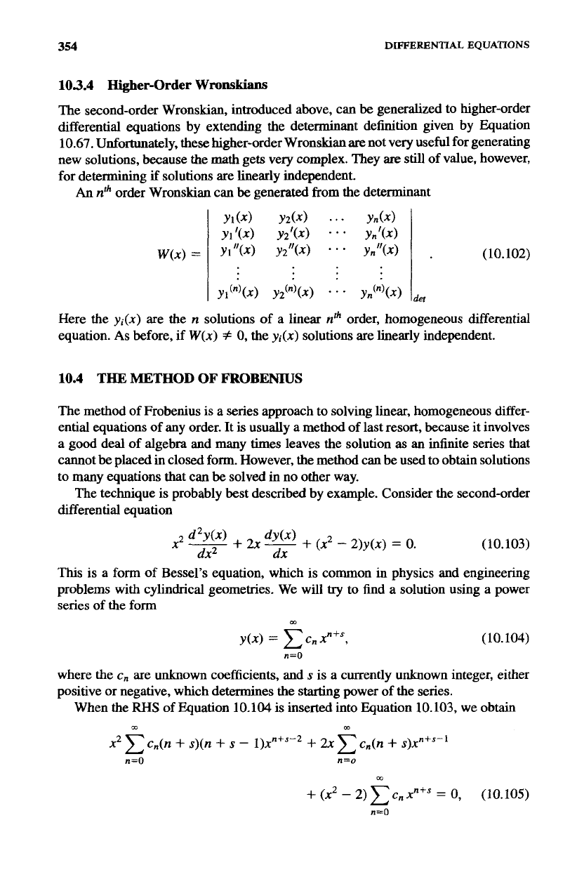
354
Ylb)
Y2W
.**
Yn(x)
Yl'(4
YZ'(X)
.
*
*
Yn'(X)
W(x)
==
Yl'W
y2"W
* * *
y,"(x)
Yl("'(X) Yz'"'(4
*
. .
Yn'"'(X)
(10.102)
det
10.4
THE
METHOD OF
FROBENIUS
The method
of
Frobenius
is
a series approach to solving linear, homogeneous differ-
ential equations of any order.
It
is usually a method
of
last resort, because it involves
a good deal of algebra and many times leaves the solution
as
an infinite series that
cannot be placed
in
closed form. However, the method can be
used
to obtain solutions
to
many equations that can
be
solved in no
other
way.
The technique is probably best described by example. Consider the second-order
differential equation
(10.103)
This
is a form of Bessel's equation, which is common
in
physics and engineering
problems with cylindrical geometries. We will
try
to find a solution using a power
series
of
the
form
m
y(x)
=
CC,X"+S,
(10.104)
n=O
where the
c,
are unknown coefficients, and
s
is a currently unknown integer, either
positive or negative, which determines the starting power of the series.
When the
RHS
of Equation
10.104
is
inserted into Equation
10.103,
we obtain
m
oc
x2
c
c,(n
+
s)(n
+
s
-
l)xn+s-Z
+
2x
c
c,(n
+
s)x"+s-'
n=O
n=o
m
+
(2
-
2)
c
c,
x"+s
- -
0,
(10.105)
n=O
THE METHOD
OF
FROBENIUS
355
where we have differentiated the series for
y(x)
term by term.
This
approach is valid
if the resulting series converges uniformly, a condition that must
be
checked once
s
and the
cn
are determined.
The terms can now be grouped based on the powers of
x
they contain:
Equation 10.106
is
of the form
Camp
=
0.
(10.107)
m
The only way the
LHS
of
this
equation can be zero for all
x
is to have all the
a,
coefficients equal to zero.
To
isolate the various powers
of
x
and their coefficients,
rewrite Equation 10.106 as
m
m
CC,
[(n
+
s)(n
+
s
-
1)
+
2(n
+
S)
-
21
x~+~
+
~C,-~X”+~
=
0.
(10.108)
n=O
n=2
The first
series
in Equation 10.108 has powers
of
x
starting with
xs,
i.e.,
xs, xS+’,
x”~,
. .
..
The second sum has powers
of
x
starting with
2+’,
i.e.,
2+2,
2+3,
. .
..
So,
in order to group according to powers
of
x,
the first two terms
of
the first summation
in Equation
10.108
have to be written out explicitly. The remaining terms can be
written as
a
sum from
n
=
2
to
n
=
m:
c,
[(s)(s
-
1)
+
2s
-
21
xs
+
c1
[(s
+
l)(s)
+
2(s
+
1)
-
21
X’+l
=
0.
(10.109)
Each of the terms in Equation 10.109 must
be
equal to zero. The coefficients
of
the
xs
and the
xs+l
terms form what are called the indicial equations:
c,
[(s)(s
-
1)
+
2s
-
21
=
0
c1
[(s
+
l)(s)
+
2(s
+
1)
-
21
=
0.
(10.1 10)
(10.1 11)
These equations determine
s.
If Equation 10.104 is
to
generate a nontrivial solution,
the
c,
coefficients cannot all be zero. There are several approaches that all generate
the same solution. We will
start
off
by assuming that
c,
#
0.
That means in order to
satisfy Equation 10.110,
(s)(s
-
1)
+
2s
-
2
=
0.
(
10.1 12)