Kusse B.R., Westwig E.A. Mathematical Physics: Applied Mathematics for Scientists and Engineers
Подождите немного. Документ загружается.

326
LAPLACE
TRANSFORMS
with a convergence region
s,
>
3.
If
h(t)
=
f(r)g(t)
then
t>O
h(t)
=
and its Laplace transform can
be
taken directly
1
a@=-
-
s-5'
(9.84)
(9.85)
with a convergence region
s,
>
5.
using Equation 9.77 and the convolution of
This
Laplace transform
of
h(t)
and
its
convergence region
can
also
be obtained
with
GsJ:
(9.86)
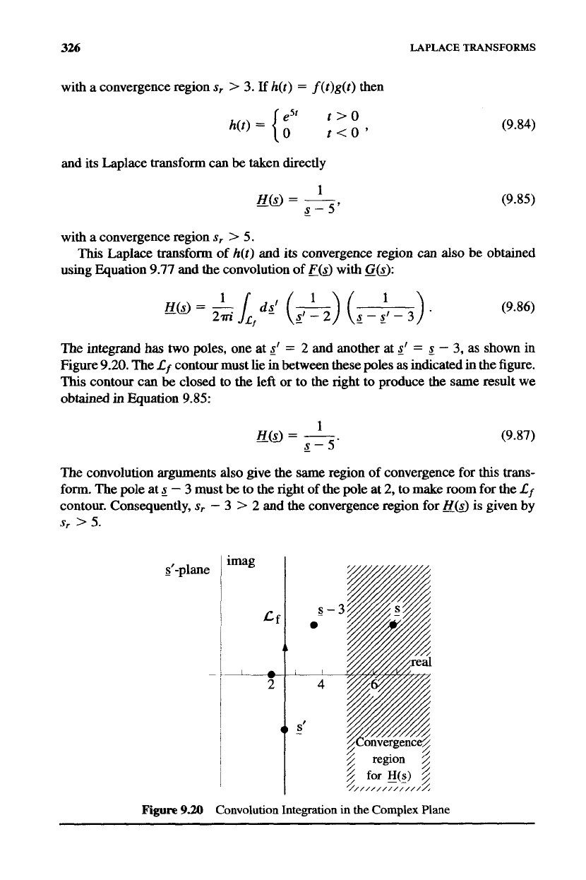
The
integrand
has two poles, one at
g'
=
2
and
another at
s'
=
g
-
3,
as shown
in
Figure 9.20. The
Lf
contour must lie
in
between these poles
as
indicated
in
the figure.
This
contour can
be
closed to the left or to the right to produce the
same
result we
obtained
in
Equation 9.85:
1
IYsJ=-
g-5'
(9.87)
The convolution arguments
also
give the same region of convergence for
this
trans-
form.
The
pole at
g
-
3
must
be
to the right of the pole at 2, to make room for the
Lf
contour. Consequently,
s,
-
3
>
2
and
the convergence region for
HsJ
is
given by
sr
>
5.
$-plane
~
!
-i
i
I
,
3
region
5
5
9
for
~(s)
$
4/////////////
Figure
930
Convolution Integration
in
the
Complex
Plane
THE LAPLACE
TRANSFORM
CIRCUIT
327
9.5.5
Summary of Transform
Properties
Some properties of the Laplace transform operation
are
summarized in the table
below. In this table the double arrow
H
is used to indicate the reversible transform
process.
9.6
THE LAPLACE
TRANSFORM
CIRCUIT
As
was the case with Fourier series and Fourier transforms, the inverse Laplace
transform can be conceptually modeled with
an
additive electronic circuit. Consider
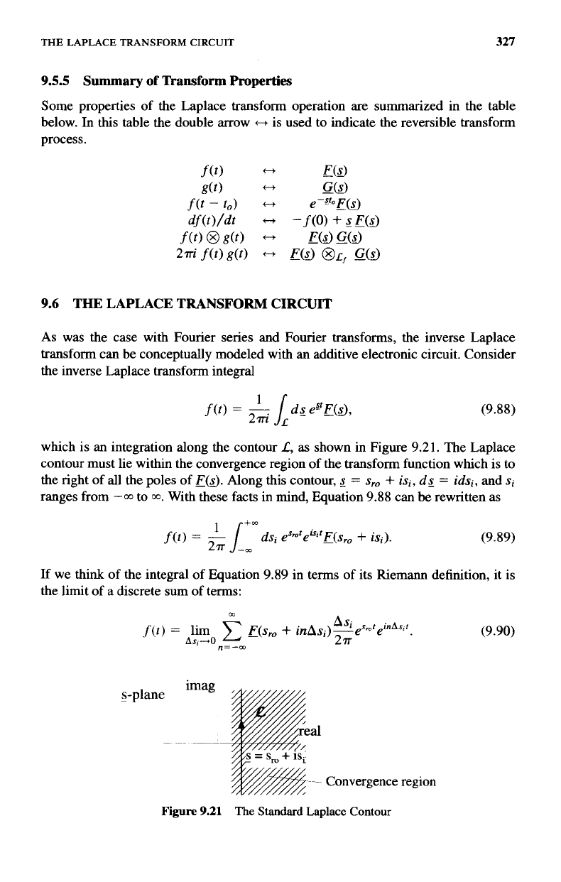
the inverse Laplace transform integral
(9.88)
which is
an
integration along the contour
L,
as
shown in Figure
9.21.
The Laplace
contour must lie within the convergence region of the transform function which is to
the right of all the poles of
EL!.).
Along this contour,
s
=
sro
+
isi,
d&
=
idsi,
and
si
ranges from
--oo
to
00.
With these facts in mind, Equation
9.88
can
be
rewritten as
f(r)
=
-L
/+mdsi
esrotefiltE(sro
+
isi).
(9.89)
If we think
of
the integral of Equation
9.89
in terms of its Riemann definition, it is
the limit of a discrete sum of terms:
27r
-m
f(t)
=
lim
2
F(s,
+
inAsi)~eSmreinAsJ
277
n=-m
As,-+O
imag
s-plane
al
-
Convergence region
Figure
9.21
The
Standard
Laplace
Contour
(9.90)
328
LAPLACE
TRANSFORMS
Equation 9.90 describes
f(t)
as
a sum of functions, each with an exponentially
growing envelope
of
(1/27r)17(sr0
+
inAsi)Asiesmr,
and oscillating as
einAsir.
9.6.1
A
Growing
Exponential
Consider the growing exponential
(9.91)
with
a
>
0.
Its Laplace transform
is
given by
(9.92)
1
-
F(S)=-.
s-a
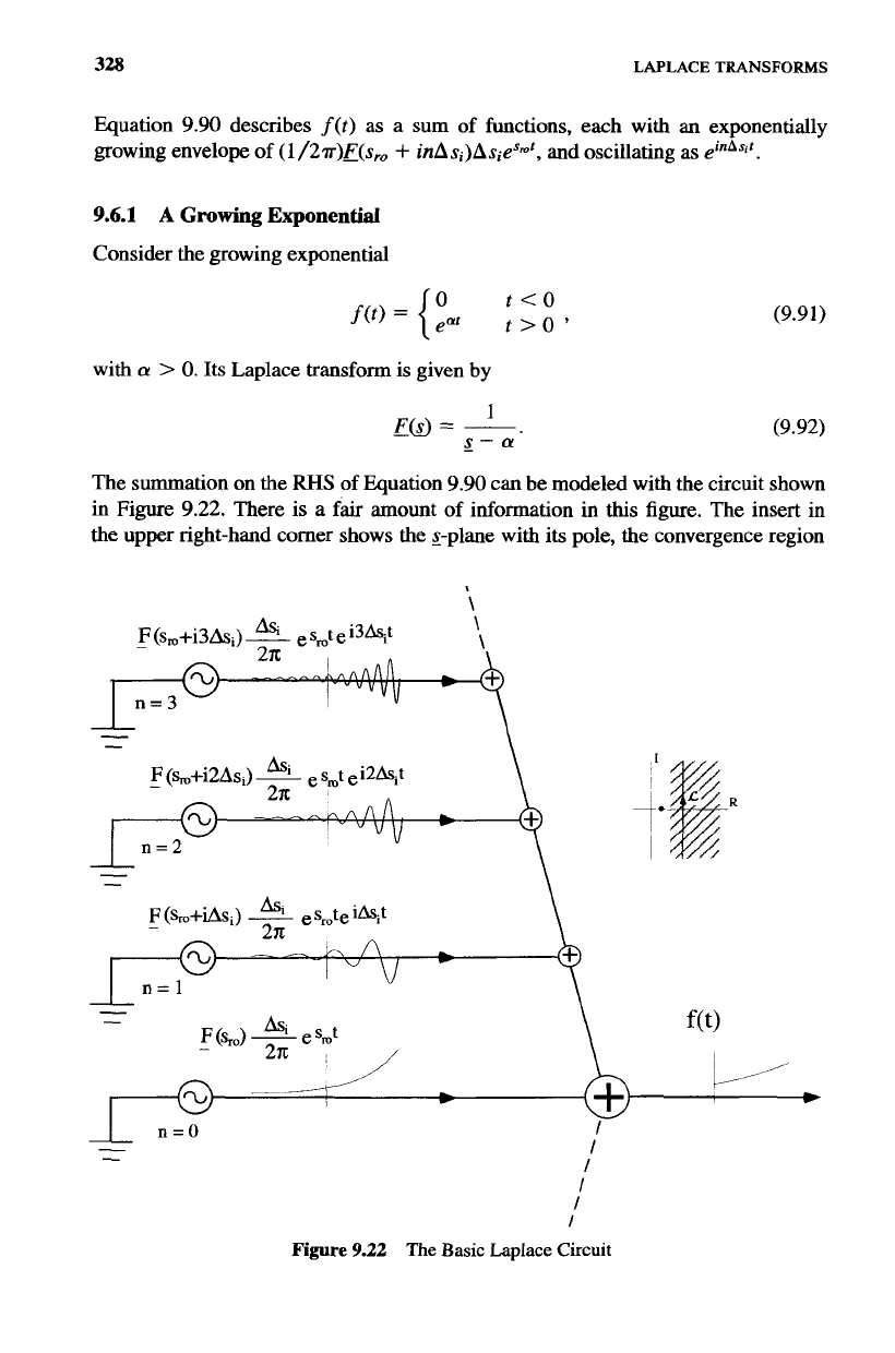
The summation on the
RHS
of Equation 9.90 can be modeled with the circuit shown
in Figure 9.22. There
is
a fair amount of information in
this
figure. The insert in
the upper right-hand comer shows the $-plane with its pole, the convergence region
\
I
I
I
I
I
I
Figure
9.22
The Basic Laplace Circuit
THE
LAPLACE
TRANSFORM
CIRCUIT
329
,
\
\
I
I
I
I
I
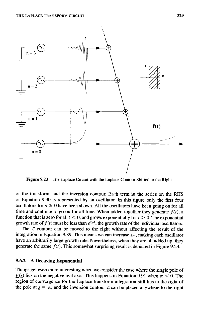
Figure
9.23
The Laplace
Circuit
with
the
Laplace
Contour
Shifted
to
the
Right
of the transform, and the inversion contour. Each term in the series on the
RHS
of Equation
9.90
is represented by an oscillator.
In
this
figure only the first four
oscillators for
n
2
0
have been shown. All the oscillators have been going on for all
time and continue to go on for all time. When added together they generate
f(t),
a
function that is zero for all
t
<
0,
and grows exponentially for
z
>
0.
The exponential
growth rate of
f(t)
must be less than
esm',
the growth rate of the individual oscillators.
The
L
contour can be moved
to
the right without affecting the result of the
integration in Equation
9.89.
This
means we can increase
sro,
making each oscillator
have an arbitrarily large growth rate. Nevertheless, when they are
all
added up, they
generate the same
f(t).
This
somewhat surprising result is depicted in Figure
9.23.
9.6.2
A
Decaying
Exponential
Things get even more interesting when we consider the case where the single pole of
F(s)
lies on the negative real axis.
This
happens in Equation
9.91
when
a
<
0.
The
region of convergence for the Laplace transform integration still lies to the right of
the pole at
s
=
a,
and the inversion contour
L
can be placed anywhere to the right
330
,
\
LAPLACE
TRANSFORMS
of
this
pole. Let’s
start
with
it
in the
right
half plane
so
that
s,
>
0.
The circuit for
this
situation is
similar
to the previous ones and
is
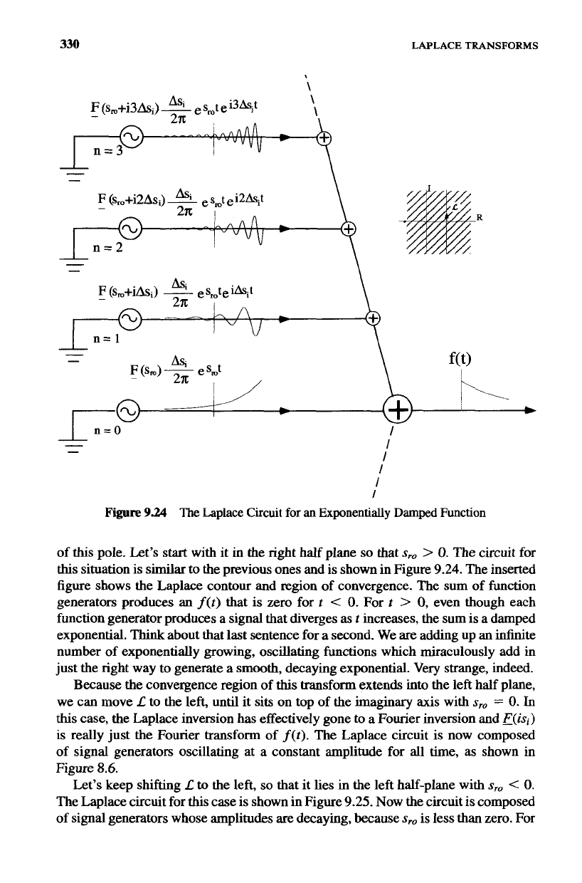
shown in Figure 9.24. The inserted
figure shows the Laplace contour and region of convergence. The sum of function
generators produces
an
f(t)
that
is
zero for
t
<
0.
For
t
>
0,
even though each
function generator produces a signal that diverges
as
t
increases, the sum is a damped
exponential. Think about that last sentence for a second. We
are
adding up
an
infinite
number of exponentially growing, oscillating functions which miraculously add in
just the right way to generate a smooth, decaying exponential. Very strange, indeed.
Because the convergence region of
this
transform extends into the left half plane,
we can move
L
to the left, until it
sits
on top
of
the imaginary
axis
with
s,
=
0.
In
this
case, the Laplace inversion has effectively gone
to
a Fourier inversion and
F(isi)
is
really just the Fourier transform of
f(t).
The Laplace circuit is now composed
of signal generators oscillating at a constant amplitude for all time,
as
shown in
Figure
8.6.
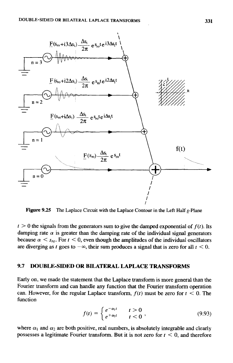
Let’s keep shifting
L
to
the left,
so
that it lies in the left half-plane with
s,
<
0.
The Laplace circuit for
this
case is shown in Figure 9.25. Now the circuit is composed
of signal generators whose amplitudes are decaying, because
s,
is less than zero. For
DOUBLE-SIDED
OR
BILATERAL LAPLACE
TRANSFORMS
331
\
L
P
\
I
I
I
I
Figure
9.25
The Laplace Circuit with the Laplace Contour
in
the
Left
Half
s-Plane
t
>
0
the signals from the generators sum to give the damped exponential
of
f(t).
Its
damping rate
(Y
is greater than the damping rate of the individual signal generators
because
a
<
s,~.
For
t
<
0,
even though the amplitudes of the individual oscillators
are diverging as
t
goes to
-a,
their sum produces a signal that is zero for
all
t
<
0.
9.7
DOUBLE-SIDED
OR
BILATERAL LAPLACE
TRANSFORMS
Early
on,
we made the statement that the Laplace transform
is
more general than the
Fourier transform and can handle any function that the Fourier transform operation
can. However, for the regular Laplace transform,
f(t)
must be zero for
t
<
0.
The
function
(9.93)
where
a1
and
a2
are both positive, real numbers,
is
absolutely integrable and clearly
possesses a legitimate Fourier transform. But it is not zero for
t
<
0,
and therefore
LAPLACE
TRANSFORMS
332
does not have a regular Laplace transform. So how can we make the claim that any
function which can be Fourier transformed can also be Laplace transformed?
It
is true that the regular Laplace transform, with the restriction that
f(t)
must be
zero for
t
<
0,
cannot handle a function like the one in Equation 9.93. However,
a
small modification to the regular Laplace transform clears up
this
problem.
Consider the Laplace transform
type
operation
(9.94)
where
t
<
0
is
now included in the integration, and
f
(t)
is given by Equation 9.93.
The obvious question immediately arises.
Is
there is
a
region of convergence in the
s-plane where the integral
of
Equation 9.94 exists? Inserting Equation 9.93
into
9.94
gives
EsJ
=
Lmdt
e-s'ea*'
+
Lrn
dt
e-S'e-al'
The first term on the
RHS
of
Equation 9.95 converges for
s,
<
a2,
and the second
term converges for
sr
>
-
a1
.
Therefore
(9.96)
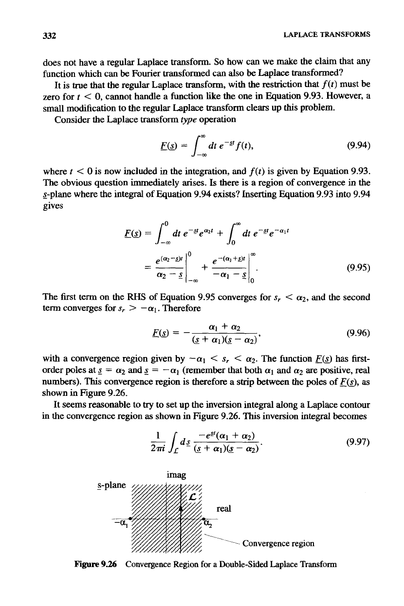
with a convergence region given by
-a1
<
s,
<
a2.
The function
E(S)
has first-
order poles at
s
=
a2
and
s
=
-a1
(remember that both
a1
and
a2
are positive, real
numbers).
This
convergence region is therefore a
strip
between the poles of
EN,
as
shown in Figure 9.26.
It seems reasonable to
try
to set up the inversion integral along a Laplace contour
in the convergence region
as
shown in Figure
9.26.
This
inversion integral becomes
(9.97)
-eJ'(al
+
a2)
1
(s+cu*)@-cu2)'
imag
1
Convergence
region
Figure
9.26
Convergence Region
for
a
Double-Sided Laplace
Transform
>OUBLE-SIDED
OR
BILATERAL LAPLACE TRANSFORMS
\
333
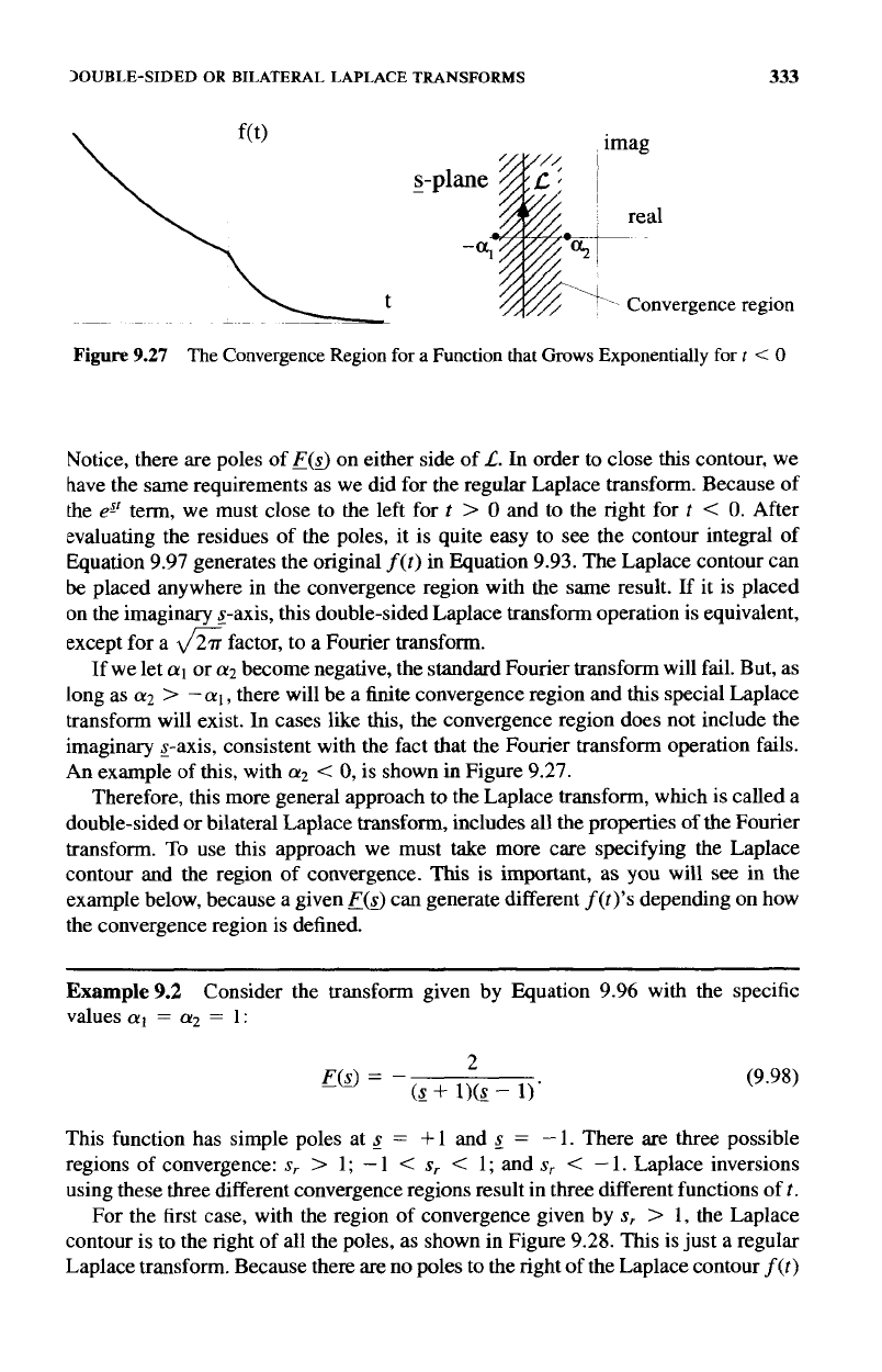
Figure
9.27
The
Convergence Region
for
a
Function
that
Grows
Exponentially
for
t
<
0
Notice, there are poles
of
f(sJ
on either side of
L.
Zn
order to close this contour, we
have the same requirements as we did for the regular Laplace transform. Because
of
the
epr
term, we must close to the left for
t
>
0
and to the right for
r
<
0.
After
evaluating the residues
of
the poles, it is quite easy to see the contour integral
of
Equation 9.97 generates the original
f(t)
in Equation 9.93. The Laplace contour can
be
placed anywhere in the convergence region with the same result. If it is placed
on the imaginary
?-axis,
this double-sided Laplace transform operation is equivalent,
except for a
&%
factor, to a Fourier transform.
If
we let
a1
or
a2
become negative, the standard Fourier transform will fail. But, as
long as
a2
>
-
a1,
there will be a
finite
convergence region and
this
special Laplace
transform will exist. In cases like
this,
the convergence region does not include the
imaginary z-axis, consistent with the fact that the Fourier transform operation fails.
An example of this, with
a2
<
0,
is shown
in
Figure 9.27.
Therefore, this more general approach to the Laplace transform, which is called a
double-sided or bilateral Laplace
transform,
includes
all
the properties
of
the Fourier
transform.
To
use this approach we must take more care specifying the Laplace
contour and the region
of
convergence.
This
is
important, as you will
see
in
the
example below, because a given
E(d
can generate different
f(t)'s
depending on how
the convergence region is defined.
~ ~~ ~ ~
Example
9.2
values
ayl
=
cy2
=
1:
Consider the transform given by Equation 9.96 with the specific
2
EM=-
(g
+
1)(s.
-
1)'
(9.98)
This function has simple poles at 8
=
+
1
and
5
=
-
1.
There are three possible
regions of convergence:
s,
>
1
;
-
1
<
s,
<
1
;
and
s,
<
-
1.
Laplace inversions
using these three different convergence regions result in three different functions
oft.
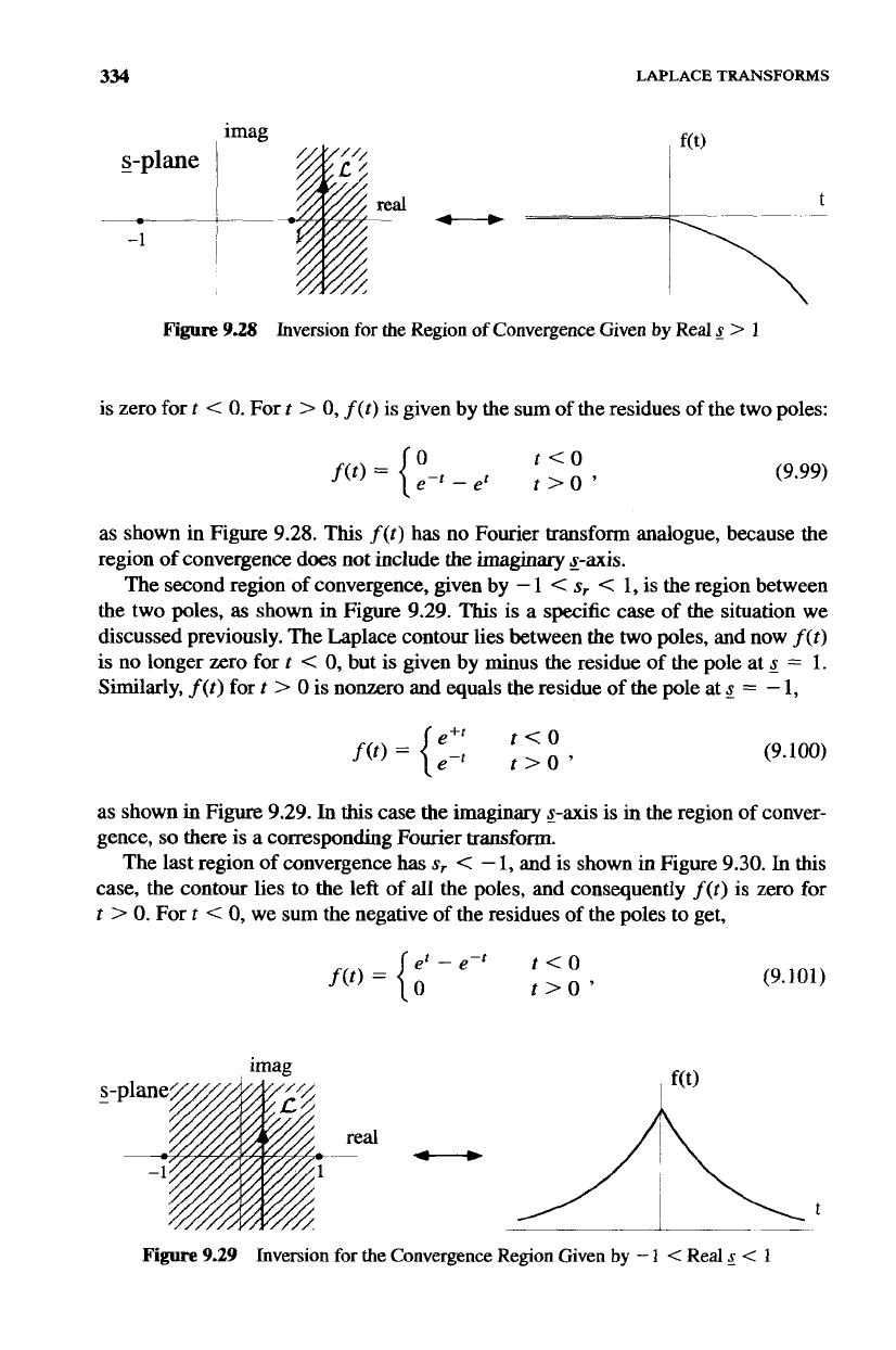
For the first case, with the region of convergence given by
s,
>
1,
the Laplace
contour is to the right of all the poles, as shown in Figure 9.28.
This
is
just
a regular
Laplace transform. Because there are no poles to the right of the Laplace contour
f(t)
334
-
s-plane
-1
LAPLACE TRANSFORMS
Figure
9.28
Inversion
for
the Region
of
Convergence Given
by
Real
s
>
1
is
zero for
t
<
0.
For
t
>
0,
f (t)
is
given by the sum
of
the residues of the two poles:
(9.99)
as
shown in Figure 9.28.
This
f(t)
has no Fourier transform analogue, because the
region
of
convergence does not include the
imaginary
x-axis.
The second region
of
convergence, given by
-
1
<
s,
<
1, is the region between
the two poles,
as
shown
in
Figure 9.29.
This
is a specific case
of
the situation we
discussed previously. The Laplace contour lies between the
two
poles, and now
f
(t)
is
no
longer zero for
t
<
0,
but is given by minus the residue
of
the pole at
8
=
1.
Similarly,
f(t)
for
t
>
0
is nonzero and equals the residue of the pole at
8
=
-
1,
(9.
loo)
as shown
in
Figure 9.29.
In
this
case the imaginary
x-axis
is
in
the region
of
conver-
gence,
so
there
is
a
corresponding Fourier transform.
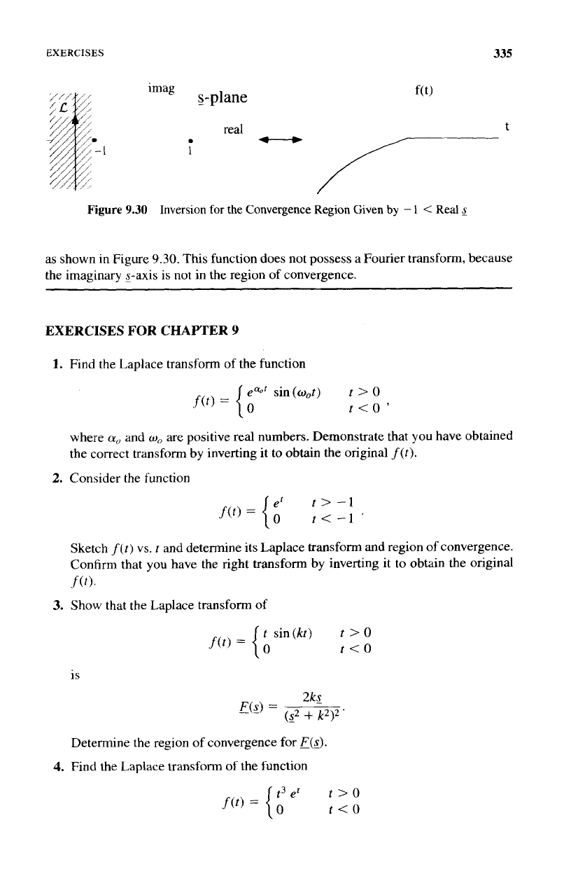
The last region of convergence
has
s,
<
-
1,
and
is
shown
in
Figure 9.30.
In
this
case, the contour lies to the left of all the poles, and consequently
f(t)
is zero
for
t
>
0.
For
t
<
0,
we sum the negative
of
the residues of the poles to get,
f(t)
=
{;
-
e-f
t<O
t>O’
(9.101)
Figure
9.29
Inversion
for
the Convergence Region Given
by
-
1
<
Real
<
1
EXERCISES
335
imag
$-plane
real
t
-1
1
Figure
9.30
Inversion
for
the Convergence Region Given
by
-
I
<
Real
2
as shown
in
Figure
9.30.
This function does not possess a Fourier transform, because
the imaginary x-axis is not in the region of convergence.
EXERCISES
FOR
CHAPTER
9
1.
Find the Laplace transform of the function
where
a,
and
w,
are positive real numbers. Demonstrate that
you
have obtained
the correct transform
by
inverting it to obtain the original
f(t).
2.
Consider the function
Sketch
f(t)
vs.
r
and determine its Laplace transform
and
region
of
convergence.
Confirm that
you
have the right transform by inverting it to obtain the original
f
(t>.
3.
Show that the Laplace transform of
t
sin(kt)
t
>
0
t<O
is
2kg
=
(s2
+
k2)2’
Determine the region
of
convergence
for
F(s).
4.
Find the
Laplace
transform of the function
t3
e‘
t
>
O
f@)={o
r<O