Kusse B.R., Westwig E.A. Mathematical Physics: Applied Mathematics for Scientists and Engineers
Подождите немного. Документ загружается.

4%
INTEGRAL
EQUATIONS
As
we did before, we will change
x
--f
x’
and then apply the operator
1
dx‘
to both sides of Equation 12.23 to give
(12.25)
The
(dy/dx)lo
term on the
LHS
is
a constant, but it is not one
of
the boundary
conditions. We label
it
as
the constant
y&
but remember that
it
is
not yet known. We
integrate again, by transforming
x
-+
x“,
and applying the operator
[
dx“
to
both sides to obtain
(12.27)
The quantity
y(0)
is one
of
the boundary conditions. Setting
y(0)
=
0
and using the
double integral identity
of
Equation
12.17
gives
(12.29)
We are not
finished
yet, because the constant
yh
is not known.
Also,
we have not
made use
of
the second boundary condition at
x
=
1.
These two things are taken care
of
at once by evaluating Equation 12.29 at
x
=
1:
I
y(l)
-
y;
+
kq
dx‘(1
-
x’)y(x’)
=
0.
(12.30)
0
Because
y(
1)
=
0,
this
equation allows
y:
to be evaluated as
1
y;
=
k,’
1
dX’(1
-
x‘)y(x’).
(12.31)
Equation 12.29 becomes
1
y(x)
=
kzx
h
dx’(1
-
x’)y(x’)
-
k,’
(12.32)
This
is clearly an integral equation.
All
the differential operators have been removed,
and both
the
boundary conditions have been incorporated. The unknown function
appears both inside and outside the integral operations, but one integral
has
constant
THE CONNECTION BETWEEN DIFFERENTIAL AND INTEGRAL EQUATIONS
497
limits and the other has the independent variable
as
an upper limit.
This
appears to
be a mixture of a Fredholm equation of the second kind and a Volterra equation of
the second kind.
A
bit more work clears up this confusion.
The integration from
x’
=
0
to
x‘
=
1 can
be
broken up into two parts. Because
the independent variable
x
ranges from
0
to 1, Equation 12.32 can be rewritten as
y(x)
=
kz
1’
dx’x(l
-
x’)y(x’)
+
ki
dx’x(1
-
x’)y(x’)
6’
-kz
lx
dx’(x
-
x’)y(x’).
(12.33)
The two integrals from
x’
=
0
to
x’
=
x
can be combined:
y(x)
=
k:
1‘
dx’x’(
1
-
x)y(x’)
+
k,”
dx’x(
1
-
x’)y(x’).
(12.34)
I’
Equation 12.34 is now in the form of a Fredholm equation of the second kind:
y(x)
=
k,’
/
~
dx’k(x, x’)y(x’),
Jo
with
x’(1
-x)
OIx’5x
x(l
-
x’)
x
5
x’
5
1
.
k(x,x’)
=
(12.35)
(12.36)
Notice that the independent variable
x
is a constant inside the integral operation,
while the
x’
is the variable of integration.
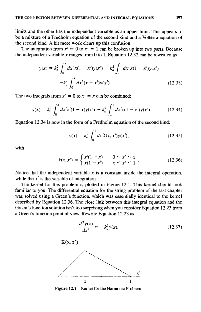
The kernel for this problem is plotted in Figure 12.1.
This
kernel should look
familiar to you. The differential equation for the string problem of the last chapter
was solved using a Green’s function, which was essentially identical to the kernel
described by Equation 12.36. The close link between this integral equation
and
the
Green’s function solution isn’t too surprising when you consider Equation 12.23 from
a Green’s function point of view. Rewrite Equation 12.23 as
(12.37)
X
1
Figure
12.1
Kernel
for
the
Harmonic
Problem
498
INTEGRAL
EQUATIONS
If
the
RHS
of
this
equation
is
looked at
as
the drive, then the Green’s function solution
for
y(x)
can
be
written
as
where
operator. That
is,
g(x15)
is
the solution of
is the Green’s function associated with the
d2y(x)/dx2
differential
(12.39)
with the same homogeneous
boundary
conditions as
y(x)
g(0lS)
=
g(115)
=
0.
(12.40)
This
Green’s function solution, Equation 12.38,
is
in the form of
an
integral equation
for
y(x).
It
is
identical to the integral equation we obtained by converting the original
differential equation, Equation 12.37,
to
an integral equation with
g(xlx’)
=
-k(x,x’).
(12.41)
12.3
METHODS
OF
SOLUTION
In
this
section, several methods of solution for integral equations are presented. The
different forms
of
integral equations generally require different solution techniques.
For example, one takes a different approach for Volterra equations of the first kind
than for Fredholm equations of the second kind.
In
these discussions,
it
is useful
to
define two classifications
of
kernels, which
we dub “translationally invariant” and “causal” kernels.
A
translationally invariant
kernel has the form
k(x,x’)
=
k(x
-
x’).
(12.42)
The motivation for
this
terminology is fairly evident, when you consider the con-
nection with the Green’s function kernels we discussed in the previous section. For
a translationally invariant kernel,
if
the drive is displaced by a certain amount, the
response will not change
its
character, but
will
just be displaced by the same amount.
A
causal
kernel
obeys
the
condition
k(x,x’)
=
0
x
<
XI,
(12.43)
which again using the Green’s function analogy, means that a response does not occur
before the drive. Several of
our
solution techniques require kernels which obey one
or
both
of these conditions.
METHODS
OF
SOLUTION
499
12.3.1 Fourier
Transform
Solutions
Recall, the standard Fourier transform operation is defined by the pair of expressions
F(w)
=
-
sp_
dt e-'"f (t)
(12.44)
Jm
do
ei"E(w).
(12.45)
A
Fourier transform approach works well for finding solutions to Fredholm equations
of the first kind, which have both translationally invariant kernels and infinite limits
of
integration:
f(t)
=
Jz.r
(1 2.46)
In
this
expression,
f(t)
and
k(t
-
7)
are known functions, and
y(t)
is unknown.
Assume that the Fourier transform of each of these functions exists:
(12.47)
(12.48)
(12.49)
Notice, because the kernel is translationally invariant, we can describe its argument
using only a single variable.
Because Equation 12.46 is a convolution of
k(t)
and
y(t),
its Fourier transform is
easy to evaluate:
Solving for
r(
w)
gives
The solution
of
y(t)
can now be obtained with a Fourier inversion:
12.3.2 Laplace
Transform
Solutions
(12.51)
(12.52)
The Laplace transform approach works for solving Volterra equations of the first kind
with causal, translationally invariant kernels and integration limits that range from
500
INTEGRAL
EQUATIONS
7
=
0
t0
7
=
f:
f(t)
=
pk(t
-
7)y(7).
(12.53)
Again,
f(t)
and the kernel are known functions, while
y(t)
is
the unknown. We assume
f(f),
y(t),
and
k(t)
are all zero for
t
<
0
and possess the Laplace transforms
(12.54)
(12.55)
(12.56)
Recall that the standard Laplace operation is defined by the equation pair
rm
E(sJ
=
/o
dte-”’f(t)
(12.57)
(12.58)
with the Laplace contour
L
to the right of all the poles of
Fb).
As it stands now, the integral in Equation 12.53 is not a convolution integral
because the upper limit of the integration is
t
rather
than
infinity. This can easily
be corrected, since we assumed a causal
kernel.
Because
k(t
-
7)
=
0
for
t
<
T,
we can extend the upper limit of the integral to
+w
without changing the value of
the integral. Because
y(~)
is zero for
T
<
0
the lower limit can be extended
to
-w
without changing the value:
f(t)
=
ldTk(f
-
‘T)Y(T)
=
dTk(t
-
7)y(7).
(12.59)
The integral equation is now in the form of a standard convolution and applying
1:
the Laplace transform operation
to
both sides gives
Solving for
Y
(g)
gives
The solution for
y(t)
is obtained with a Laplace inversion:
(12.61)
(12.62)
In this expression, the Laplace contour must be to the right of all
the
poles of the
quantity
EWKOl.
METHODS
OF
SOLUTION
501
12.3.3
Series
Solutions
Fredholm equations of the second kind can be solved by developing what is known as
a Neumann series solution.
In
quantum mechanics, this process is called perturbation
theory. The general form
of
a Fredholm equation of the second kind is
y(x)
=
f(x)
+
A
dx’k(x,x’)y(x’),
Ib
(12.63)
where
f(x)
and
k(x,
x’)
are known functions,
A
is a constant, and
y(x)
is the unknown.
The constant
A
is assumed to be “small” in some sense.
To
start, we will assume
that
A
is small enough that
(12.64)
for all
a
<
x
<
b.
This really does not pin down the magnitude of
A
very well, because
the integral on the
RHS
of
Equation
12.64
cannot be evaluated without knowing
y(x)
in advance. Notice how
f(x)
cannot be zero anywhere. If it were, Equation
12.64
could never be satisfied, regardless of the magnitude of
A.
Colloquially, we describe
this requirement by saying the method requires a nonzero “seed’ function.
If
Equation
12.64
is satisfied, an iterative approach can be employed to obtain a
solution for
y(x)
to arbitrary orders of
A.
As
a first approximation, the solution can
be given by
We call this the zerorh-order solution because
A
does not appear in this expression. An
improvement on this approximate solution
is
made if we substitute the zerorh-order
solution into the integral of Equation
12.63
and then solve for a new value of
y(x):
(12.66)
We call
y1
(x)
the first-order solution, because it has a term with
A
raised to the first
power. Now you probably see what we are doing.
To
get the second-order solution,
we substitute
y1
(x)
back into Equation
12.63
and solve for
a
new
y(x):
YZ(X)
=
f(x)
+
A
dx’k(x,x’)yl(x’)
I”
b
=
f(x)
+
A
dx’k(x,x‘)f(x’)
(12.67)
b
+A2
lb
dx’k(x,
x’)
.I
d~”k(x’,
x”)f(x”).
INTEGRAL
EQUAnONS
502
And of course, you guessed
it,
this
is called a second-order solution because the
highest power
of
A
that appears is
A2.
This
process can be canied to any order. The
@-order solution is
(12.68)
+
h2
Lb
dxrlb
dx“
k(x,
x‘)k(x‘,
x“)
f
(x“)
In
this
expression
x”‘
is used to indicate
an
x
with
n
primes.
Now
our
hope is that
y(x)
=
lim
yn(x).
(12.69)
That is,
if
we
keep performing the iterative process of substituting our approximate
result for
y(x)
back into the equation, we will eventually converge on the correct
solution. The standard convergence tests should be applied to check that the resulting
infinite sum converges. Obviously,
A
must be
small
enough for
this
to
occur.
n-m
Example
12.2
Most engineering and physics problems formulate naturally as dif-
ferential equations
as
opposed to integral equations. That is why more emphasis, in
this
book and in others, is placed on solutions to differential equations rather than
integral equations. There are some problems, however, that do formulate naturally
as
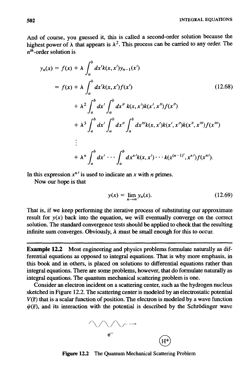
integral equations. The quantum mechanical scattering problem is one.
Consider an electron incident on a scattering center, such
as
the hydrogen nucleus
sketched in Figure
12.2.
The scattering center
is
modeled by an electrostatic potential
V(i)
that is
a
scalar function of position. The electron is modeled by a wave function
$(F),
and its interaction with the potential is described by the Schrodinger wave
WA-
-
e-
Figure
12.2
The
Quantum
Mechanical Scattering
Problem
503
METHODS
OF
SOLUTION
equation:
(12.70)
Here
E
is the energy of the electron and
m
is its mass. If we define the constant
k2
=
2mE/h2, Equation 12.70 can
be
rewritten as
2m
h2
(V2
+
k2)
+(F)
=
-V(F)+(i-).
(12.71)
This last equation is a linear differential equation with
+(I;)
as the dependent variable.
A
Green's function approach to solving
this
equation gives the result
(1
2.72)
The first term on the
RHS
is the solution for
+(F)
when
V(F)
is zero, the homogeneous
version of Equation 12.71. The second term is
an
integral over all space involving
the Green's function
g(F1i').
The Green's function itself is a solution to
(V2
+
k2)
g(FIF')
=
S3(F
-
P).
(12.73)
It will be assumed that the Green's function vanishes at infinity. Applying this bound-
ary
condition gives
(12.74)
If
$(F)
were not sitting inside the Green's function integral of Equation 12.72, we
would already have our desired solution. But since it does appear both inside and
outside of the integral, we resort to the Neumann series method described earlier. The
potential
V(F)
is assumed to be a small perturbation to the problem. The zero-order
solution is just the wave function for a free electron
+o(f)
=
eik.r
(12.75)
We obtain the first-order solution by forcing this solution back into Equation 12.72:
(12.76)
This solution is referred to as the first
Born
approximation. Higher-order approxirna-
tions follow the Neumann series solution method.
You may have noticed something a little odd about
this
example. In the derivation
of the Neumann series, the constant
A
needed to be small enough for the series
to converge. In this example, however, the constant
A
is nowhere
to
be seen. The
convergence of this solution is controlled by the magnitude of
V(i-).
504
INTEGRAL EQUATIONS
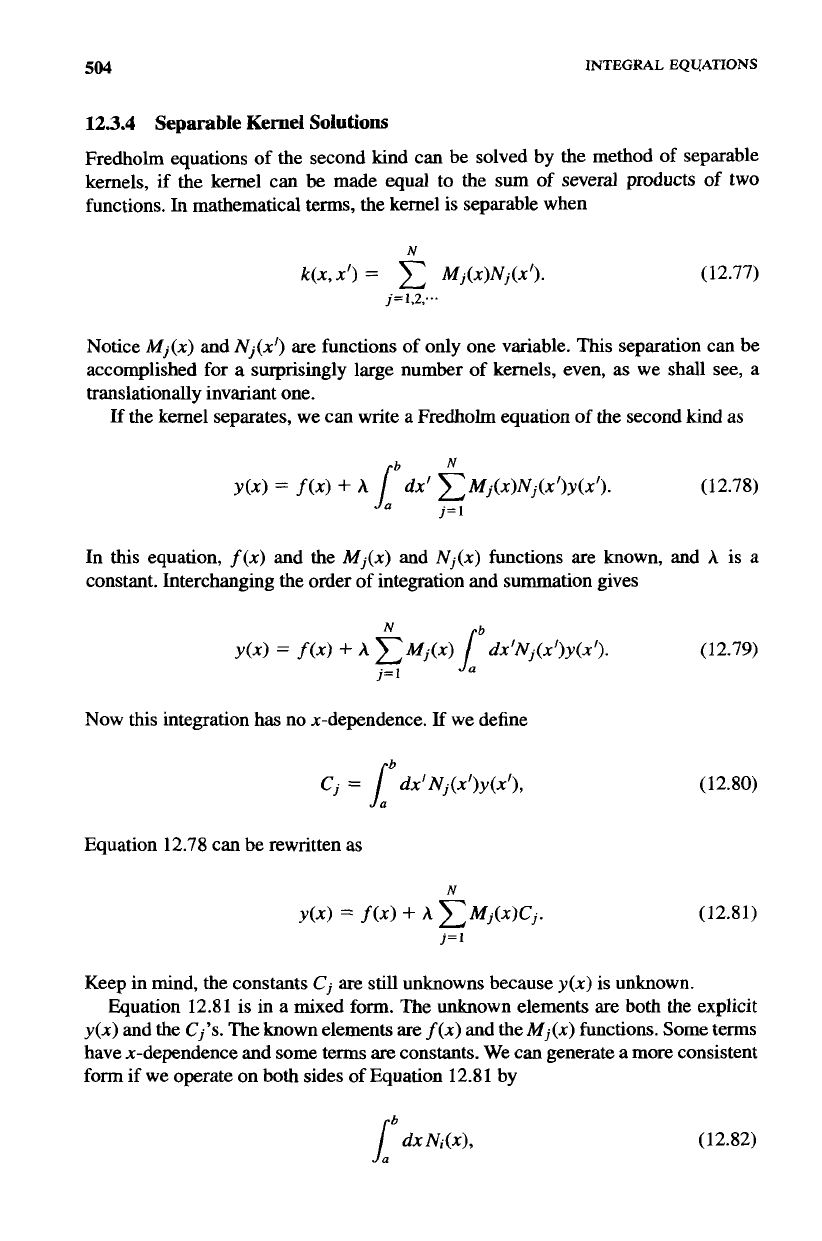
12.3.4
Separable
Kernel
Solutions
Fredholm equations of the second kind can be solved by the method
of
separable
kernels, if the kernel can
be
made equal to the
sum
of several products
of
two
functions.
In
mathematical terms, the kernel is separable when
N
k(x,x’)
=
c
Mj(X)Nj(X’).
(12.77)
Notice
M,(x)
and
Nj(x’)
are functions of only one variable.
This
separation can be
accomplished for a surprisingly large number
of
kernels, even, as we shall see, a
translationally invariant one.
If
the kernel separates, we can write
a
Fredholm
equation
of
the second kind as
y(x)
=
f(x)
+
h
dx‘ cMj(x)Nj(x’)y(x’).
(12.78)
I”
j:l
In
this
equation,
f(x)
and the
Mj(x)
and
Nj(x)
functions are known, and
h
is
a
constant. Interchanging the order of integration and summation gives
Now
this integration has no x-dependence.
If
we define
b
cj
=
dX”j(X’)Y(X’),
(12.79)
(12.80)
Equation 12.78 can be rewritten as
Keep in mind, the constants
Cj
are
still unknowns because
y(x)
is unknown.
Equation 12.81 is in a
mixed
form. The unknown elements are both the explicit
y(x)
and the
Cj’s.
The known elements are
f(x)
and theMj(x) functions. Some terms
have x-dependence and some terms
are
constants. We can generate a more consistent
form
if
we operate
on
both sides of Equation 12.81 by
(12.82)
METHODS
OF
SOLUTION
505
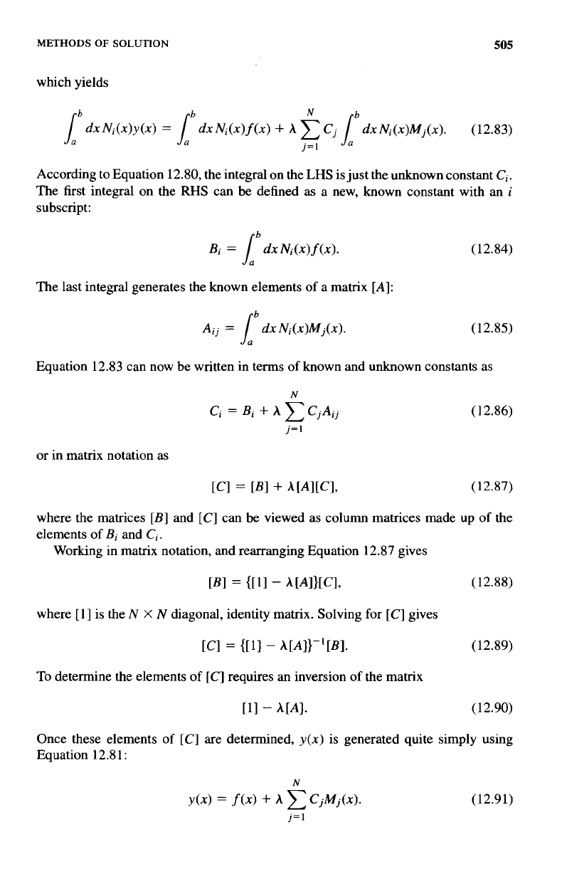
which yields
According to Equation 12.80, the integral on the
LHS
is just the unknown constant
Ci.
The first integral on the
RHS
can be defined
as
a new, known constant with an
i
subscript:
6
Bi
=
dxN;(x)f(x).
The last integral generates the known elements
of
a matrix
[A]:
(12.84)
(12.85)
Equation 12.83 can now be written in terms
of
known and unknown constants as
N
C,
=
B;
+
A
CjAij
j=
1
(12.86)
or in matrix notation as
where the matrices
[B]
and
[C]
can be viewed as column matrices made
up
of the
elements
of
Bi
and
C,.
Working in matrix notation, and rearranging Equation 12.87 gives
where [l] is the
N
X
N
diagonal, identity matrix. Solving for
[C]
gives
[CI
=
m1
-
"l)-"Bl.
(12.89)
To determine the elements
of
[C]
requires an inversion
of
the matrix
[I1
-
AM].
(12.90)
Once
these elements of
[C]
are determined,
y(x)
is generated quite simply using
Equation 12.81:
N
(12.91)
j=1