Kusse B.R., Westwig E.A. Mathematical Physics: Applied Mathematics for Scientists and Engineers
Подождите немного. Документ загружается.

506
INTEGRAL EQUATIONS
This
matrix notation points out a very interesting result for these types
of
problems.
If
f(x)
=
0,
then all the elements of the
[B]
matrix are also zero. Therefore, from
Equation 12.88, it can be seen that a nonzero
[C]
matrix, and therefore a nonzero
y(x),
can exist only
if
Given the
[A]
matrix, Equation 12.92 will
be
satisfied only for specific values of
A.
A
nonzero solution to the original integral equation will exist only for these
An
eigenvalues, and the solutions
yn(x)
are
eigenfunctions of the integral equation:
(12.93)
1
An
lb
dx’k(x,
x’)
yn(~’)
=
-yn(X).
Example
123
It is possible to separate kernels that do not appear, at first glance,
to be separable.
As
an example, consider the translationally invariant kernel
k(t,t’)
=
cos(t
-
t’).
(12.94)
This kernel can be separated with the trigonometric identity
cos(t
-
t’)
=
cos(t) cos(t’)
+
sin(t) sin(t‘),
(12.95)
so
that
L
cos(t
-
t’)
=
xMj(t)Nj(t‘),
j=
1
where
Ml(t)
=
cos(t)
Mz(t)
=
sin(t)
Nl(t’)
=
cos(t’)
N2(t’)
=
sin(t’)
(12.96)
(12.97)
EXERCISES FOR CHAPTER
12
1.
2.
Derive the Fredholm integral equation that corresponds to
subject to the boundary conditions
y(1)
=
y(-
1)
=
0.
How does the integral
equation change
if
the boundary conditions are changed to
y(
1)
=
dy/dxl
=
l?
Convert the following integral equation to a differential equation:
y(x)
=
[dx’(x2
-
xx’)y(x’).
EXERCISES
507
Identify all the boundary conditions included
in
the integral equation, which
must be specified to make the solution to the differential equation unique.
3.
Given the Fredholm equation of the second kind,
where
x)(t
+
1)/2
(1
-
t)(x
+
1)/2
-1
<
t
<
x
x
<
t
<
1
k(x,t)
=
{
('
-
'
obtain the associated second-order differential equation and the boundary con-
ditions.
4.
Convert the integral equation
Y(X)
=
1
-
x
f
dt
(X
-
t)y(t)
l
to a differential equation, with the appropriate boundary conditions.
5.
Convert the integral equation
+(x)
=
1
+
h2
[
dt
(x
-
t)+(t)
to a differential equation and determine the appropriate boundary conditions.
6.
Use Fourier techniques to solve the following Fredholm integral equation for
4
(x)
:
7.
Use Laplace techniques to solve the following integral equation
for
+(x):
8.
Using the Neumann series approach, solve
to obtain
+(x)
=
epx2
508 INTEGRAL
EQUATIONS
9.
Consider the Fredholm equation
(a)
Using the method of separable kernels, determine the values for
h
which
(b)
Determine all the nonzero solutions for
+(x).
allow solution for
+(x).
10.
Consider the differential equation
dx
+
A;x2y(x)
=
0,
with the boundary condition
y(0)
=
1.
(a)
Convert
this
differential equation and its boundary condition to
an
integral
equation.
(b)
Using the Neumann series approach, obtain a solution to the integral equation
assuming small
A,.
Can you place
this
solution in closed form, Le., not in
terms
of
an
infinite series?
11.
Solve
+(x)
=
x
+
dt
(1
+
xt)+(t)
I’
by
three methods,
(a)
the Neumann series technique.
(b)
the separable kernel technique.
(c)
educated guessing.
integral equations:
12.
Find the possible eigenvalues and the eigenfunction solutions of the following
1
i.
4(x)
=
h
ii.
+(x)
=
A
ll
dt
(t
-
x)+(t)
iii.
+(x)
=
h
dt(x
-
t)’+(x).
s_,
1
1
dt(xt
+
x)+(t).
Ll
13
ADVANCED TOPICS IN
COMPLEX ANALYSIS
This chapter continues our discussion of complex variables with the investigation
of two important, advanced topics. First, the complications associated with multi-
valued complex functions
are
explored. We will introduce the concepts of branch
points, branch cuts, and Riemann sheets, which will allow us to continue to use the
residue theorem and other Cauchy integral techniques on these functions. The second
topic describes the method of steepest descent, a technique useful for generating
approximations for certain types of contour integrals.
13.1
MULTIVALUED FUNCTIONS
Up to this point, we have concentrated on complex functions that are single valued.
A
function
&)
is a single-valued function of
z
if it generates one value of
w
for a
given value of
z.
The function
-
w=z
2
(13.1)
is example of a single-valued function of
z.
In
contrast, the function
-
W=g
1
/2
(13.2)
is an example of a multivalued function of
z.
This is easy to see, because
z
=
1
generates
w
=
+
1
or
w
=
-
1.
Another point,
g
=
2i,
gives either
w
=
fi
eiTI4
or
operation is performed
only on a positive real quantity to produce a single, positive, real result. Operations
like
(
)'I2
can have positive, negative, or complex arguments and produce multivalued
results.
509
-
w
=
JZei5~/4.
In this chapter, we will use
the
convention that the
510
ADVANCED
TOPICS
IN
COMPLEX ANALYSIS
13.1.1
Contour Integration
of
Multivalued
Functions
In
Chapter
6,
special techniques were derived for performing integrals in the complex
plane. Can we still use the residue theorem and the other Cauchy integral techniques
on these multivalued functions? The answer is yes,
if
we are careful!
From our previous work, we know that if the complex function
I&)
is analytic
inside
a
closed contour
C.
we can
write
(13.3)
The key requirement here is that
the
contour must
be
closed. For
this
path to be closed,
the variable of integration
g
has
to return to its starting value. For a single-valued
function,
this
obviously
also
brings
~(g)
back to its starting value. The same is not
always true with a multivalued function, and
this
is the source of some difficulties,
as you will
see
in the
two
examples that follow.
Example
13.1
The single-valued function
-
W=$
(13.4)
is analytic everywhere in the complex
z
plane. Remember, for a function to be
analytic, we must
be
able to write
w
=
u(x,
y)
+
iv(x,
y),
with
u(x,
y)
and
v(x,
y)
being continuous, real functions that obey the Cauchy-Riemann conditions. In
this
case,
and
(13.5)
(13.6)
So
the Cauchy-Riemann conditions are satisfied for all
g.
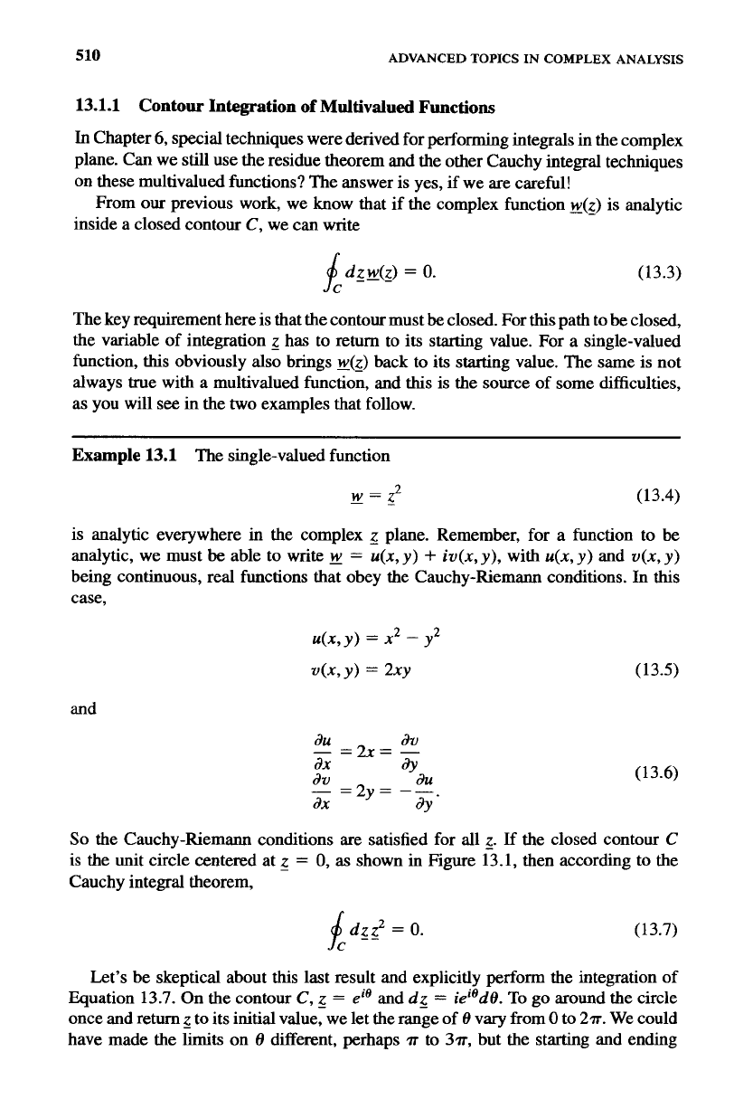
If
the closed contour
C
is the unit circle centered at
z
-
=
0,
as
shown in Figure 13.1, then according to the
Cauchy integral theorem,
f
dgg
=
0.
C
(13.7)
Let’s be skeptical about
this
last result and explicitly perform the integration of
Equation
13.7.
On
the contour
C,
g
=
eie
and
dg
=
ieiedO.
To
go
around the circle
once and return
g
to its initial value, we let the range
of
8
vary from
0
to
27~.
We could
have made
the
limits
on
8
different, perhaps
T
to 37r, but the starting and ending
MULTIVALUED
FUNCTIONS
Y
-
z-plane
511
Figure
13.1
Contour
for
Unit Circle Integration
values of
8
must differ by
27r
so
the circle is traversed exactly once. The integral
becomes
=
(1/3)(ei6"
-
1)
=
0,
(13.8)
which is exactly the expected result. The integral around a closed path of this analytic
function is zero. There are no surprises here.
Example
13.2
Now consider the multivalued function
(13.9)
The single point
simple way to see this is to write
z
-
using an exponential representation
=
1
will give two different values for
y:
w
=
1
and
w
=
-
1.
A
Notice that all these expressions identify the point
g
=
1, but do
so
using different
polar angles.
Now
use the fact that
(ei')3/2
=
e3'l2
to
obtain the corresponding values
of
y:
1
-1
,iO
=
&67r
=
ei12.rr.
. .
=
-
w={
or (13.11)
,i3n
=
,i97r
=
ei15.rr.
.
.
=
Two different values for
w
are generated by
this
process.
512
ADVANCED
TOPICS
IN
COMPLEX
ANALYSIS
Is
this
function analytic? If we write
z
-
=
x
+
iy,
we have
-
w
=
(x
+
iyl3l2,
(13.12)
and with
w
=
u(x,
y)
+
iu(x, y),
1
2-
1 1
2i 2i
u(x,y>
=
-(w
+
w*)
=
(x
+
iy)3/2
+
(x
-
iy)3/2]
V(X,Y)
=
--(klI
-
w*)
=
-
[(x
+
iy)3/2
-
(x
-
i~)~/'].
(13.13)
The partial derivatives become
(1 3.14)
and
so
the Cauchy-Riemann conditions
are
satisfied for all
g.
Ths means the function
given
in
Equation
13.9
is analytic everywhere in the g-plane, and consequently its
closed line integral around the
unit
circle shown in
Figure 13.1
should
be
zero:
(13.15)
Again, let's be skeptical about
this
result and check it explicitly by performing
the same type of integration worked out in the previous example.
As
before, we set
z
-
=
,i@
,
dg
=
ieiedO,
and let
0
range from zero to
2a:
6'"
(13.16)
J
4
5'
=--
Uh-oh! The Cauchy integral theorem appears to be violated.
Our
function
is
analytic
inside
C,
but the integral is nonzero. Because
the
Cauchy integral theorem is the
basis for complex integration using the residue theorem, its violation would
be
a big
problem. Fortunately, there is a way to preserve the validity of the theorem.
MULTIVALUED FUNCTIONS
513
Notice, although the
0
to 27r range of
8
returns
z
to its starting value in the above
integration, it does not return
g
to its initial value. When
8
=
0,
z
=
eiO
=
1
and
g=
1,butwhen8=27r,z=ei2"= 1andw=ei3"=
-
-1
.
B
ut if we go around
the unit circle
twice,
that is
0
<
8
<
4~r,
both
z
and
~(z)
=
g312
will return to their
starting values, and we obtain
It appears that the definition of closed integral contour must take on new meaning
when we are using multivalued functions.
We
cannot say a contour is closed unless
both the variable of integration and the function being integrated simultaneously
return to their initial values. We will investigate
this
idea in detail in the sections that
follow.
13.1.2 Riemann Sheets, Branch Points, and Branch
Cuts
Branch points, branch cuts, and Riemann sheets are all concepts developed
so
that
the Cauchy integral theorem, the residue theorem, and all the other tools developed
for analytic functions will still work with multivalued, complex functions.
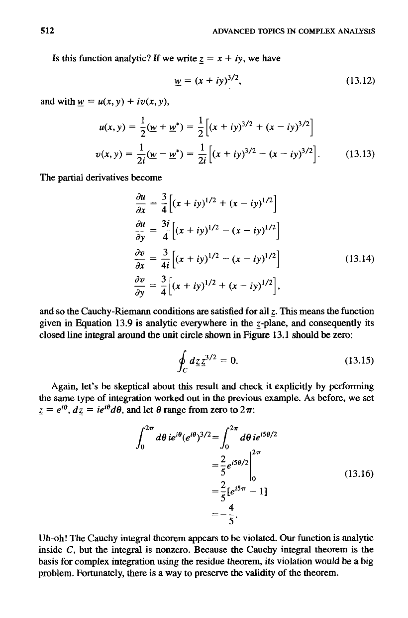
Riemann Sheets
looking at their mapping properties. Consider the simple function,
The nature of multivalued functions can
best
be explained by
-
w(z)
=
z1'2.
(
13.18)
It is easy to see this function is multivalued. The single point
z
=
eim14
=
ei9"14
maps
onto two different points in the y-plane,
w
=
ei"l8
and
211
=
ei9"18.
This mapping is
shown in Figure 13.2.
Y
a
X
-
z-plane
V
a
U
-
a
y-plane
Figure
13.2
Mapping
of
a Multivalued
Function
514
z-plane
3x
Y
X
Figure
133
ADVANCED TOPICS IN COMPLEX ANALYSIS
V
y-plane
"?
V
V
Mapping
of
y
=
gl/*
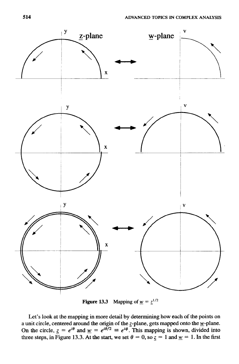
Let's
look
at
the mapping in more detail
by
determining how each
of
the points
on
a unit circle, centered around the origin
of
the z-plane, gets mapped onto the w-plane.
On the circle,
z
=
eie
and
=
eie/*
=
ei+.
This
mapping
is
shown, divided into
three steps, in Figure
13.3.
At the
start,
we set
8
=
0,
so
z
=
1
and
y
=
1.
In
the first
MULITVALUED
FUNCTIONS
515
pair of pictures, we see that as the polar angle
8
increases from
0
to
T,
4
increases
from
0
to
~/2.
So
w
moves along its own unit circle, lagging
z
in angle by a factor
of two. In the middle pair of pictures,
8
continues to increase from
T
to
2~,
so
that
z
returns to
z
=
ei2=
=
1, its initial value. However,
ends up at
w
=
eiV
=
-
1,
because
4
has only increased
to
T.
In the last pair of pictures,
8
continues to increase
from
2~
to
4~,
repeating the loop it has already made, and once again returns to its
initial value ofz
=
ei4=
=
1. At the
same
time,
w
finally makes a complete circle
and returns to its initial value,
w
=
ei2=
=
1.
With
the interpretation that a closed
contour in the Z-plane must return both
z
and the function
~(g)
to their starting values,
the unit circle in the Z-plane must be traversed twice in order to form a closed path
for the function
=
$I2.
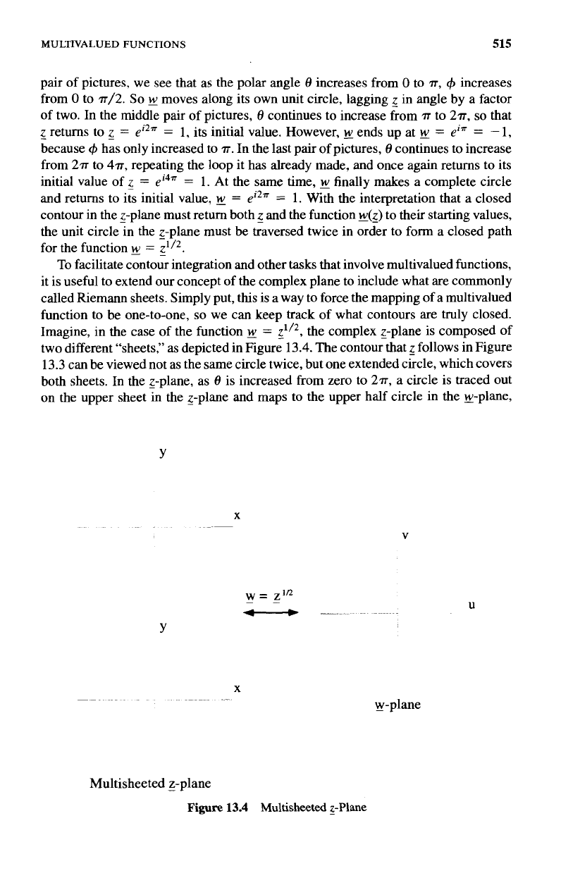
To
facilitate contour integration and other tasks that involve multivalued functions,
it is useful to extend our concept of the complex plane to include what are commonly
called Riemann sheets. Simply put, this is a way to force the mapping of a multivalued
function to be one-to-one,
so
we
can
keep track
of
what contours are truly closed.
Imagine, in the case of the function
w
=
z1I2,
the complex g-plane is composed of
two different “sheets,” as depicted in Figure 13.4. The contour that follows in Figure
13.3 can be viewed not as the same circle twice, but one extended circle, which covers
both sheets. In the 2-plane, as
8
is increased from zero to
2m,
a circle is traced out
on the upper sheet in the 2-plane and maps to the upper half circle in the !?-plane,
Y
Y
X
y-plane
Multisheeted ?-plane
Figure
13.4
Multisheeted
g-Plane