Lehner G. Electromagnetic Field Theory for Engineers and Physicists

Подождите немного. Документ загружается.

64 Basics of Electrostatics

by which the surface element is seen from the field point. The element of the

solid angle is the projection of the surface element onto a unit sphere centered

about the field point, as illustrated in Fig. 2.21. It can be calculated by eq. (2.70).

Consequently, and are dimensionless quantities. This definition is in

analogy to that of the “plane” angle (see Section 2.5.4, on line dipoles and in

particular Fig. 2.29, which is the equivalent of Fig. 2.21 for that case).

The result is

(2.71)

Specifically, for a surface with uniform surface density of the dipole moment we

find

(2.72)

where is the solid angle under which the uniform dipole layer appears when

looking from the field point. Confusion with the electric flux (for which was

also used) should not be an issue.

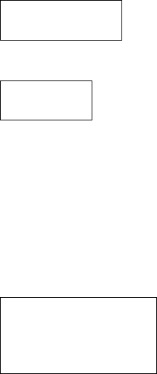
As an example, let us consider a sphere whose surface is uniformly covered

with outwardly facing dipoles. We may picture this uniform dipole layer as

consisting of two concentric spheres with opposite charges, where the charge is

very large and the difference of their radius is very small. For all points inside the

sphere we have (the negative sign is a result of the definition of in

Fig. 2.20). Conversely, for all points outside we have . Therefore (for

outwardly oriented dipoles) we get

(2.73)

When passing through the dipole layer from inside to outside, the potential

experiences a discontinuity by .

This result can be generalized. It applies to a dipole layer of any shape and is

independent of whether is uniform or not. Passing through a dipole layer in the

direction of the dipole increases the potential by , where is now a function

of the location. The potential difference depends on how one passes through the

dipole layer. One proves this generalized claim by beginning with a surface that is

covered with electric charges. Let the surface charge density at a particular point be

and the electric displacement just above that point be , and the one

underneath . One can split and into their parallel (tangential) and

perpendicular (normal) components with respect to the surface (Fig. 2.22).

Now, one applies eq. (2.4) to the small cylinder shown in Fig. 2.22 whose extent

perpendicular to the surface shall be so small that the contribution of the sides of

the cylinder vanishes. The remaining contribution is

A'd

dΩ

dΩΩ

4πε

------------

τdΩ

∫

4πε

------------

Ω =

Ω

Ω 4π–= θ

Ω 0=

-----– inside

0 outside











τε

⁄

τε

⁄τ

σ D

2.5 The Ideal Dipole 65

(2.74)

Notice that we did not make any statement about the tangential components, here,

which will be covered in a later section. Now consider the case of two parallel

surfaces in close vicinity with surface charges of opposite sign (Fig. 2.23), for

which one finds:

From these two equations it follows:

and

Therefore, the normal component of D remains unchanged by the dipole layer. The

normal component of D within the layer is decreased by the value of . The

voltage when passing through the layer in perpendicular, positive direction is:

Fig. 2.22

dA–

–()dA σdA=

– σ =

Fig. 2.23

+σ

-σ

– σ–=

–+σ=

σ–=

66 Basics of Electrostatics

(2.75)

As before, the positive direction is the direction of the dipole moment. is finite,

while d is arbitrarily small and is large enough to make finite, i.e., precisely

(2.76)

With eq. (2.75) we obtain for the potential difference or voltage

(2.77)

which completes the proof.

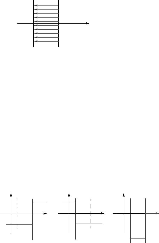
Particularly simple is the case of two infinitely wide parallel planes with

homogeneous surface charges (Fig. 2.24). For symmetry reasons, D has an x-

component depending on x only. Fig. 2.25 illustrates (a) the field of a surface with

the surface charge , (b) the field of a surface with the surface charge , and

For symmetry reasons

δϕ E

d–

---------

d–

σ–

----------------

d–== =

σσd

σd τ=

δϕ

σd

------

-----==

Fig. 2.24

+σ-σ

+σ -σ

Fig. 2.25

+σ

-σ

---=

---–=

---=

---–=

+σ

σ–=

(a)

(b) (c)

– σ=

–=

2.5 The Ideal Dipole 67

(2.78)

For case (b), in a similar way one obtains

(2.79)

The superposition gives a non-zero field only for the area between the two planes

and it points from the positive plane to the negative one (Fig. 2.24)

(2.80)

Therefore

(2.81)

and

(2.82)

This equation is exact even for finite distances d, while for the general case, i.e.,

when deriving eq. (2.75), an infinitesimal distance d was required.

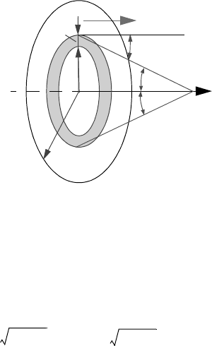
Here is another example on how to apply eq. (2.72). To calculate the potential

at the axis of a disk, uniformly coated with dipoles (Fig. 2.26). One needs to find

the solid angle . From eq. (2.70), follows for z>0:

Now, substituting as a new variable. Then and thus

–

---==

–

---–==

σ–=

-----–=

δϕ E

d–

σd

------

-----===

Fig. 2.26

Ω

Ω dΩ

∫

2πr

----------------

θcos rd

∫

2πr

----------------

zrd

--------------------

∫

2πz

rrd

-----------------------

∫

2rdr=

68 Basics of Electrostatics

For z < 0, on the other hand,

There is a discontinuity at z = 0, where jumps from to ,

which results in an overall discontinuity of , as expected. The electric field on

the axis is

and is calculated to be

vanishes when approaches infinity, as necessary. Now, we come back to the

case of Fig. 2.24, for which the field is non-zero only inside the layer.

Ωπz

-----------------------

∫

πz

--------------------–

2π 1

--------------------–







2π 1 θ

cos–()==

Ω 2π 1

--------------------–







–2π 1–

--------------------–







2ε

--------

--------------------–







for z 0>

2ε

--------

1–

--------------------–







for z 0<











ϕτ2ε

()⁄– τ 2ε

()⁄

τε

⁄

z∂

∂ϕ

–=

2ε

--------

-----------------------

2.5 The Ideal Dipole 69

2.5.4 Line Dipoles

It is possible to cover lines with dipoles, which is illustrated by a simple example.

According to eq. (2.46), the potential of an infinitely long, straight line charge is

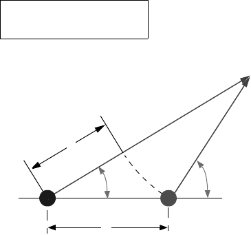
Two parallel line charges in close vicinity form a line dipole (Fig. 2.27), with the

potential

which holds as long as

We now require that

and

Then , . Furthermore , and

because the power series of for ,

becomes

(2.83)

Fig. 2.27

-q

2πε

------------

-----ln–=

2πε

------------

-----ln–

2πε

------------

-----ln+=

2πε

------------

-----ln–

2πε

------------

δ–

-------------ln–==

2πε

------------

----–





ln–=

θ≈≈ δ r

– d θ r

«cos⋅≈= r

r≈≈

1 x–()ln xx

2⁄…++()–=1x 1≤≤– ϕ

2πε

------------

qd() θcos

2πε

-----------------------

≈≈

70 Basics of Electrostatics

where (qd) is the line dipole density (dipole moment per unit length) and is the

potential of the infinitely long line dipole. The result should be compared to

eq. (2.60), which represents the potential of a dipole. When comparing with

eq. (2.60), replace p with (qd), use 2

instead of 4

, r instead of r

, and let

. We should keep in mind that r in eq. (2.60) represents the distance of the

field point from the dipole, while in eq. (2.83) r represents the perpendicular

distance to the line dipole.

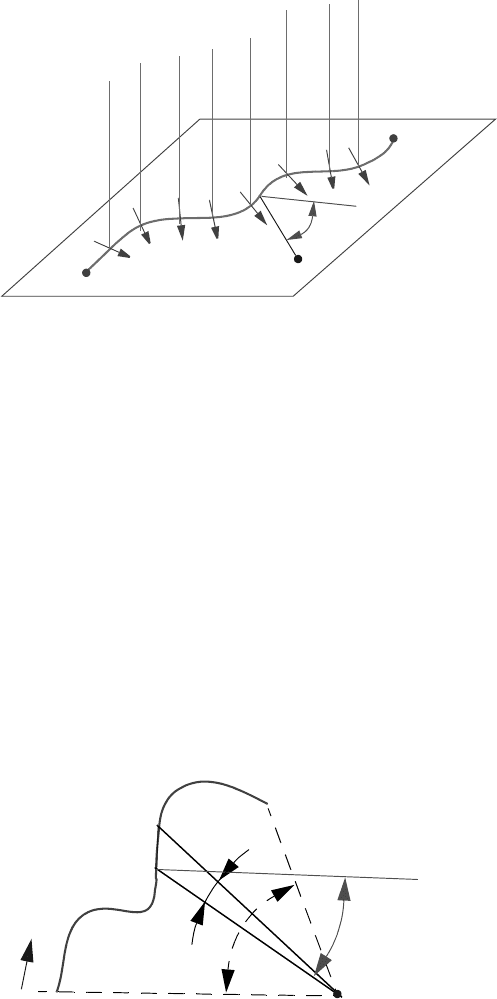
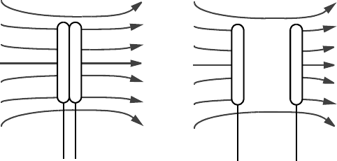
From line dipoles that are parallel to each other, one can construct cylindrical

dipole layers (Fig. 2.28 and Fig. 2.29 ).

The surface density of the dipole moment is

and thus the potential becomes

Fig. 2.28

Fig. 2.29

dα

τ s()

dqd()

--------------=

τθcos ds

2πε

---------------------

∫

2.5 The Ideal Dipole 71

where the integral from A to B is evaluated along the contour C. Now,

is the angular element, under which the line element ds appears when looking from

the field point. Therefore

(2.84)

If is constant, this gives

(2.85)

These two relations are equivalent to eq. (2.71) and eq. (2.72), respectively. There,

we discussed general spatial problems, while here we are dealing with the

cylindrical case, which is also called the plane case because it is independent of

one of the spatial coordinates.

When the contour C is closed, the result is a closed cylinder. If, furthermore,

is constant and the dipoles point outwardly, then

and thus

As expected, there is the discontinuity of the potential .

dα

θcos ds

------------------=

2πε

------------

τdα

∫

τα

2πε

------------

2π– inside

0 outside







-----– inside

0 outside.











τε

⁄

72 Basics of Electrostatics

2.6 Behavior of a Conductor in an Electric Field

One finds in nature two quite distinct types of materials. There are materials

containing charges which can move freely and there are materials where this is not

the case. The former are called conductors, while latter are called insulators (or

dielectrics). Consider the behavior of materials in the presence of an electric field

for the case of a conductor. We refrain from discussing this broad classification

further, but limit our discussion to the consequences for conductors in an electric

field, and then tackle the problem of dielectrics in an electric field.

A conductor in an electric field experiences a force, which is actually exerted

on the free charges within it. These start to move, and their motion will cease only

everywhere inside the conductor and

(2.86)

The surface of the conductor has to have the same potential everywhere, i.e. it has

to be an equipotential surface. Outside of the conductor, will not vanish. Its

tangential component has to be zero at the conductor surface

(2.87)

as otherwise the surface would not be an equipotential surface. The perpendicular

component of , however, will not vanish. There will be surface charges at the

surface, such that the external field does not penetrate the conductor, i.e., by

eq. (2.74) we obtain

(2.88)

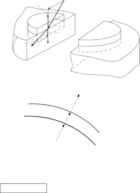
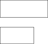
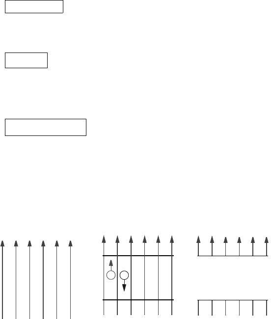
To illustrate this, consider this simple example: We choose an infinitely wide,

conducting plate within a uniform electric field which is perpendicular to the

surface of the plate (Fig. 2.30). Depending on their sign, the free charges move in

the direction of the field or opposite to it, until they reach the surface of the plate.

This is so, regardless of whether there are only negative, positive, or both types of

charges available. The result is a surface charge which is positive on one end, and

Fig. 2.30

σε

abc

++++++

------

σε

E–=

E 0=

ϕ const =

0 =

σ ==

2.6 Behavior of a Conductor in an Electric Field 73

negative on the other. The inside is free of any field if . The field of the

surface charges exists only inside. It originates at the positive charges (sources) and

ends at the negative charges (sinks). i.e., it is exactly opposite to the external field

but of the same magnitude. The external field is thus identically cancelled. The

superposition of the fields of Fig. 2.30b and Fig. 2.24 results in Fig. 2.30c.

The thereby created surface charges are also called influence charges. They

can be used to measure the electric field by magnitude and direction. A pair of

conducting plates does the job. The plates are brought into the field while in

contact with each other. In the field, they are separated, and by trying different

orientations, one can find the direction of the field (Fig. 2.31).

To calculate the field created by a conductor, together with an external field in

full generality is rather difficult. In the following, we will solve some problems that

are, however, rather easy to solve.

2.6.1 Metallic Sphere in the Field of a Point Charge

By now, we have already calculated a number of fields and in principle, we know

their equipotential surfaces. One may imagine each such equipotential surface as

the surface of a conductor. In light of this, we have already solved many problems

of this kind. In Section 2.4, we have found that the equipotential surface of

two point charges with opposite sign is that of a sphere (Fig. 2.10). Take a sphere of

radius , centered at the origin of a Cartesian coordinate system, and a charge Q

to be located at (0,0,z

). Because of eq. (2.54) and eq. (2.55), a second charge Q

location (0,0,z

) will make the sphere an equipotential surface provided,

(2.89)

σε±

Fig. 2.31

ϕ 0=

-----=