Lehner G. Electromagnetic Field Theory for Engineers and Physicists

Подождите немного. Документ загружается.

74 Basics of Electrostatics

(2.90)

The charge Q

at location (0,0,z

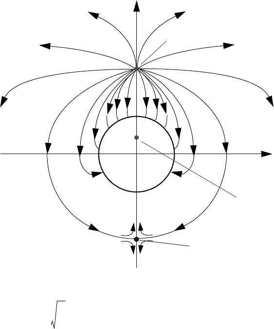
) is a fictitious or image charge. Given Q

location (0,0,z

), this image charge is necessary to create the very field outside of

the sphere that we are looking for. There is no field inside the sphere. The field

ends at the surface of the sphere at the correlating surface charges, which are

determined by equation eq. (2.88). Integration of these charges over the surface of

the sphere yields the charge Q

. On the sphere’s surface end all those field lines

which would end at Q

, the so-called image charge, if there were no sphere. The

resulting configuration is illustrated in Fig. 2.32. The point is the

image point of the point with respect to the sphere. From this stems the

term image charge and the method to solve this kind of problems is called the

method of images.

One can modify this problem slightly, and require that the sphere holds a

given charge Q. The solution results from recognizing that if one places an

arbitrary charge at the center of the sphere its surface remains an equipotential

----–=

00z

,, r

⁄=(

)

00z

,,(

)

charge Q

image charge Q

stagnation point

Fig. 2.32

2.6 Behavior of a Conductor in an Electric Field 75

surface. All we need to do is to superimpose the field of a point charge (Q - Q

) at

the center to the initial field of Fig. 2.32

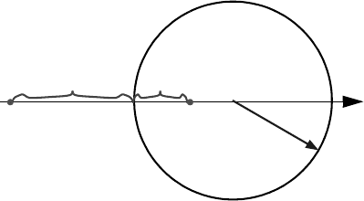
A charge in front of a plane, conducting wall represents the limit of the sphere

with an infinite radius r

. It results from eq. (2.89) that the mirror or image charge

has to be located behind the wall, in the exact same distance as the real charge in

front of it, i.e., in its image point and that . The charge location

according to Fig. 2.33 is

and, therefore by equation eq. (2.89)

If , then in the 1

approximation

that is

It is plausible that thereby the boundary condition of constant potential or

vanishing tangential field components is met at the wall (Fig. 2.34). It is also

possible to apply this method to charges inside an angle as shown in Fig. 2.35. In

this case there are the charges +Q at for example (a,b,0) and (-a,-b,0) and the

charges -Q at (-a,b,0) and (a,-b,0). One can think of the field in the 1

quadrant

(there is no field in the other ones) being generated by those four charges and it is

easy to verify that the planes xz and yz are equipotential surfaces, which is quite

plausible.

–=

Fig. 2.33

–=

–

----------------==

-----+

---------------=

– r

-----–





≈ r

–==

≈

76 Basics of Electrostatics

Of course, it is also possible to place several charges, for example, in the

vicinity of the sphere of Fig. 2.32. This requires multiple image charges, and all

fields need to be added. In particular, it is possible to add another charge -Q

(0,0,-z

) besides the charge Q

at (0,0,z

). This requires one to consider two image

charges: Q

at (0,0,z

), and another one -Q

at (0,0,-z

). In the limit of Q

and z

Fig. 2.34

-Q

Fig. 2.35

-Q

+Q -Q

2.6 Behavior of a Conductor in an Electric Field 77

approaching infinity then Q

needs to approach infinity in the same manner, while,

goes to zero. That is to say, the two image charges in the said limit result in a

dipole. The field of the two charges ±Q

in the vicinity of the sphere can be

regarded as being uniform. This suggests that the problem of a sphere in a uniform

field can be solved by means of a fictitious (image) dipole at its center. This leads

us to the next example.

2.6.2 Metallic Sphere in a Uniform Electric Field

Based on the just mentioned assumption and using the quantities from Fig. 2.36,

one makes the following Ansatz:

is the externally applied field, which at a sufficiently large distance, is not

distorted by the metallic sphere. The potential is generated by the dipole according

to eq. (2.60) and by a part that belongs to the uniform outside field. This

assumption is confirmed if we can choose p such that is constant for all :

will, in fact, be constant for , provided one chooses

Thus

(2.91)

This allows one to calculate the components of :

p θcos

4πε

----------------- E

a ∞,

z–=

p θcos

4πε

----------------- E

a ∞,

r θcos–=

a ∞,

ϕ rr

Fig. 2.36

a ∞

ϕϕ

p θcos

4πε

----------------- E

a ∞,

θcos–==

ϕ rr

4πε

a ∞,

ϕ E

a ∞,

----- r–







θcos=

78 Basics of Electrostatics

(2.92)

. (2.93)

at the surface of the sphere ( ). determines the surface charge:

(2.94)

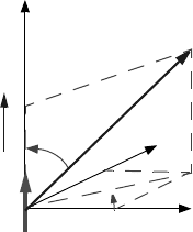
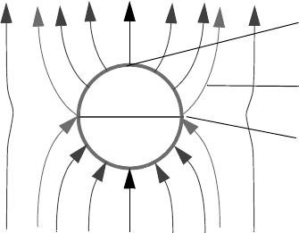
This configuration is illustrated in Fig. 2.37. The maximum field is

and is located at the two poles of the sphere. The behavior at the equator is strange,

insofar as it consists entirely of many stagnation points forming a so-called

stagnation line. The field lines there form a tip, i.e. they have no unique direction,

which is, of course, only possible at stagnation points. Furthermore, one can show

that they form an angle of 45° against the equatorial plane (Fig. 2.38).

This problem can be generalized, which gives rise to the question how this

picture might change if the sphere carried the charge Q. Thus far, the effect of the

sphere was simulated by a fictitious dipole, i.e. the charge on the sphere vanishes,

which can also be obtained when integrating σ over the surface, eq. (2.94). So, one

only needs to place an additional charge in the center of the sphere. This solves the

problem because it also creates a constant potential on the sphere.

Instead of eq. (2.91), we now use

Depending on Q, very different field configurations result, which are presented

here without proof. Consider:

a ∞,

-----







θcos=

a ∞,

-----1–







θsin=

0= rr

= E

σε

()

3ε

a ∞,

θcos===

E 3E

a ∞,

Fig. 2.37

field maximum is located

at the poles of the sphere

separatrix

stagnation points

at the equator of the sphere

(“stagnation line”)

ϕ E

a ∞,

----- r–







θcos

4πε

--------------+=

2.6 Behavior of a Conductor in an Electric Field 79

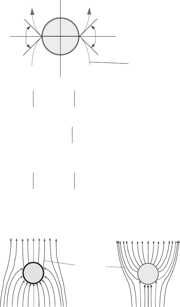
Case 1: if ,

then the stagnation lines are at circles of equal latitudes of the sphere, as shown in

Fig. 2.39.; and

Case 2: if ,

then the stagnation lines are degenerate and the stagnation points of Fig. 2.39 move

to the poles of the sphere; and

Case 3: if

then the stagnation points detach from the sphere, and move out into the field along

the axis through the poles (Fig. 2.40).

separatrix

Fig. 2.38

45°

Fig. 2.39

Q < 0

Q > 0

separatrix

4πε

a ∞,

⋅

-------------------------------------

4πε

a ∞,

⋅

-------------------------------------

4πε

a ∞,

⋅

-------------------------------------

80 Basics of Electrostatics

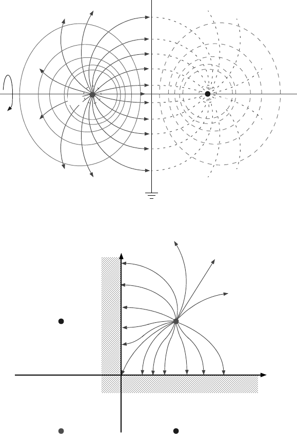
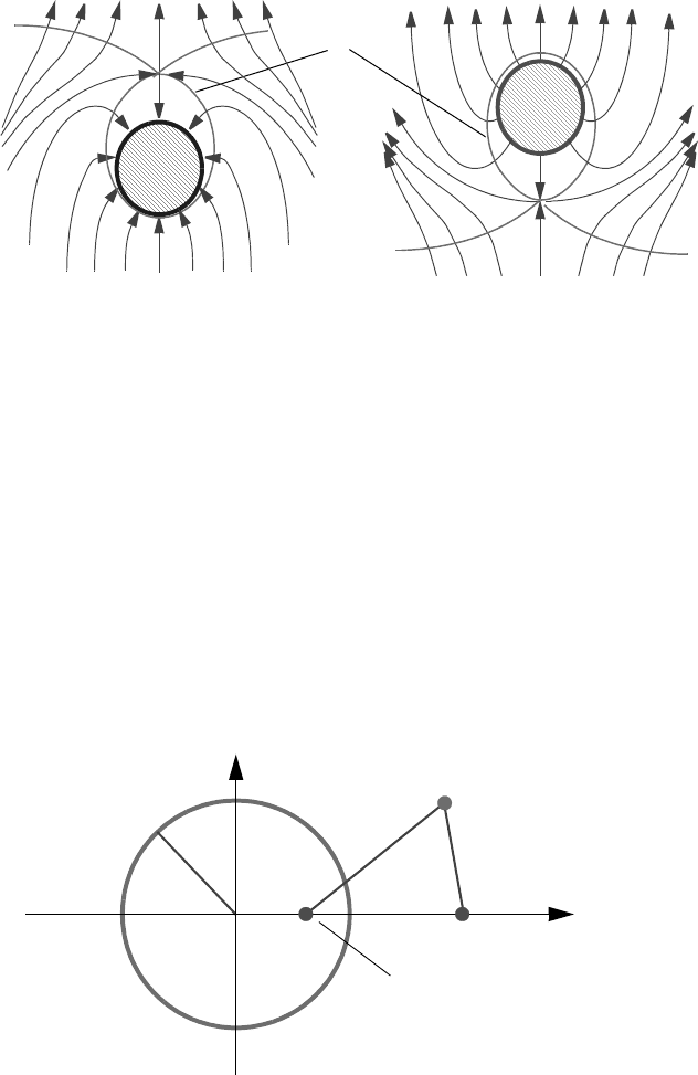
2.6.3 Metallic Cylinder in the Field of a Line Charge

Consider a metallic cylinder to be located within the field of a uniform line charge

with its axis oriented parallel to the line charge (see Fig. 2.41). One can think of the

overall field outside the cylinder as being created by the given line charge q

(outside the cylinder) and its image charge, also a line charge -q (inside). The

product of the distances of the two line charges from the cylinder axis equals the

square of the cylinder radius, i.e. the piercing points of the two line charges emerge

by reflection at the circle , (where is the radius of the cylinder). Thus

The proof is easy. Based on eq. (2.46), one first calculates the potential of the two

line charges at a field point (x,y,z)

Fig. 2.40

separatrix

(equipotential

surface

Q < 0 Q > 0

through S)

= r

⋅ r

Fig. 2.41

(x, y, z)

q (line charge)

-q

image charge (line charge)

metallic cylinder

2.7 The Capacitor 81

where

and

On the cylinder wall we have

and thus

Therefore , and thereby also are constant on the cylinder wall. The

location of all the geometrical points for which the distance ratios from the

two fixed points is constant, as shown in Fig. 2.41 These are known in geometry as

the circles of Apollonius. The circular cross section of the cylinder constitutes one

of those circles.

2.7 The Capacitor

Suppose there are two conductors (for example metals) with a charge of opposite

sign (Q and -Q), then a field will form between them whose force lines originate on

one surface and terminate on the other. Both surfaces are equipotential surfaces, i.e.

a well defined voltage V between the two bodies is set up. This voltage is

proportional to the charge Q. The ratio is a geometric factor called the

capacitance C. The whole configuration is termed the capacitor.

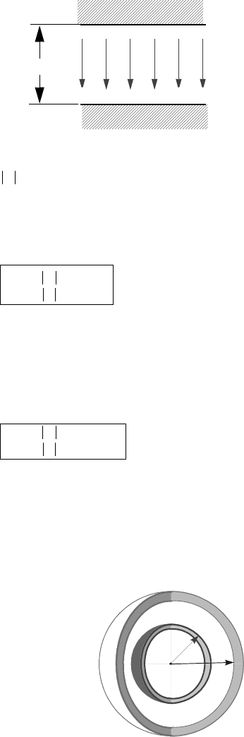
It is particularly simple to calculate the case of a plane, parallel plate

capacitor when one makes the approximation that the plates extend to infinity,

thereby neglecting fringing effects (Fig. 2.42). Then

2πε

------------

-----ln–

2πε

------------

-----ln+

2πε

------------

----ln==

–()

+ x

------–







+==

+ r

-----

2xr

------------–

------ y

2xx

– x

------------------------------------------------=

2xr

------------–

------+

2xx

– x

-------------------------------------

------ const===

⁄ϕ

⁄

QV⁄

-----=

82 Basics of Electrostatics

and

The charge is

where A is the area of the plates. Therefore

(2.95)

One could also define the capacitance of a single conductor by using the value of

its voltage against a point at infinity. Consider a sphere of radius r, with a voltage

between its surface and infinity

so that

(2.96)

Two concentric spheres form a spherical capacitor (Fig. 2.43). For this case,

the voltage is

and therefore

Fig. 2.42

++++++

------

σ–

σd

------=

Q σA±=

-------

---------

4πε

--------------=

-------4πε

r ==

Fig. 2.43

4πε

------------

---

----–





2.7 The Capacitor 83

(2.97)

If one lets and become very large, but keep to be very small,

then

and the case of the parallel plane capacitor is recovered.

Two concentric cylinders form a cylindrical capacitor. Here

and thus

(2.98)

This is exact only for a cylinder of infinite length l, which would make C also

infinite. Therefore, it is more practical to express the capacitance per unit length.

In spherical or cylindrical coordinates, the electric field has a spatial dependency

according to eq. (2.2) and eq. (2.45):

spherical cylindrical

Electric field in general

E has its maximum at the inner

electrode

Another way to write this is as

follows:

-------4πε

–

--------------

– d=

C 4πε

-----

---------==

2πε

--------------

-----





ln–

2πε

--------------

-----





ln+

2πε

--------------

----





ln==

-------2πε

----ln





1–

----2πε

----ln





1–

4πε

-----------------= E

2πε

----------------=

max

4πε

-----------------= E

max

2πε

------------------=

max

4πε

-----------------

–()

-----------------------

max

2πε

------------------

= =

----ln

---------------