Lehner G. Electromagnetic Field Theory for Engineers and Physicists
Подождите немного. Документ загружается.

114 Basics of Electrostatics
2.15 Forces in the Electric Field
2.15.1 Force on the Plate of a Capacitor
Consider, a capacitor with the charge Q, insulated from its surroundings (for
example, the charge Q remains unchanged). A charge Q within the field E,
experiences the force
.
Here, E is the field that exists without the charge Q. The electric field inside the
capacitor is
.
It would be wrong to assume that the force that one plate exerts on the other could
be calculated using this field. This field is created by the charges on both plates. We
may conclude from our discussion of Fig. 2.25, that the field of one charged plate
at the location of the other is exactly half that field, namely . The magnitude
of the force is therefore
.
(2.175)
This force is attracting since the charges on the two plates have opposite signs.
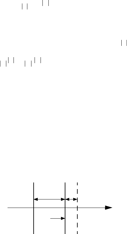
To solve this problem in a different way is also possible. We take a capacitor
with variable plate distance x. Its energy as a function of x is
.
It requires a force to increase the distance between the plates. i.e., it requires
mechanical energy to increase the plate’s separation. Neglecting friction, this work
must be found again in the electric field energy of the capacitor. For a virtual
displacement we obtain with the notation of Fig. 2.65
.
F QE=
E
1
ε
---
D
1
ε
---
σ
1
ε
---
Q
A
-------
== =
σ 2ε⁄
FQ
σ
2ε
------
Q
Q
2εA
----------
Q
2
2εA
----------== =
W
Q
2
2C
-------
Q
2
2εA
----------
x==
dx
Fig. 2.65
x
x
dx
F
x
F
x
dx– dW
Q
2
2εA
----------
dx==
2.15 Forces in the Electric Field 115
i.e.,
.
(2.176)
Besides the sign, which expresses the direction of the force, this confirms above
expression. Both methods are thus equivalent. The second method is often more
convenient. Written in a slightly different form:
.
or per unit area the force is
.
(2.177)
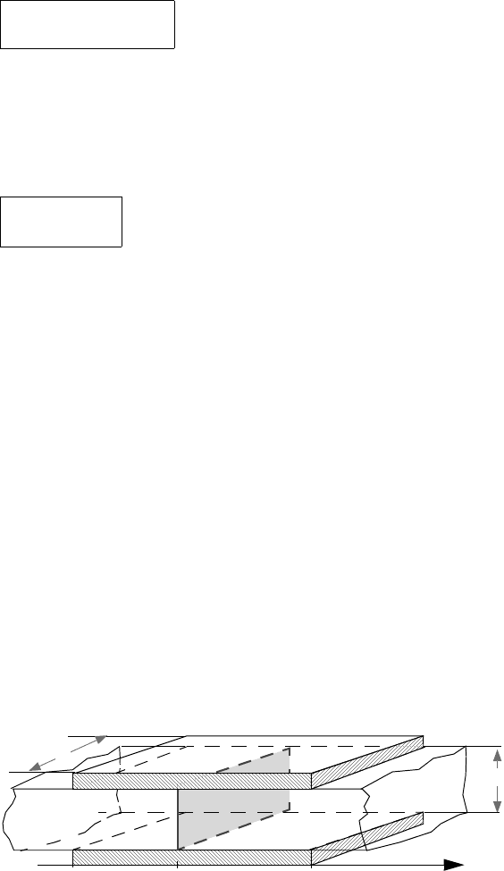
2.15.2 Capacitor with two Dielectrics
Consider the capacitor shown in Fig. 2.66, which is filled with two different
dielectrics. The question is whether or not those dielectrics exert some force on
each other. To solve this problem is easy when using the method of virtual
displacement. As before, the charge Q shall be kept constant, i.e., the capacitor is
insulated.
Then the energy of the capacitor is
.
Using
and
yields
F
x
Q
2
2εA
----------–
dW
dx
--------
–==
F
x
σ
2
A
2
2εA
-------------–
1
2
---
Aσ
σ
ε
---
–
1
2
---
ADE–== =
F
x
A
------
1
2
---
ED –=
Fig. 2.66
d
a
ε
1
ε
2
x
l
x
0
W
Q
2
2C
-------=
Q ε
1
E()ax ε
2
E()al x–()+=
VEd=
C
Q
V
----
ε
1
ax ε
2
al x–()+
d
------------------------------------------==
116 Basics of Electrostatics
and
.
This results in
,
i.e., there is a force in positive x-direction when and in negative x-direction
when . Per unit area the force is
(2.178)
where of course .
Both results, (2.177) and (2.178) indicate mechanical stress or pressure in the
form . Thus we can say, that electric fields cause mechanical stress
in the direction parallel to their field and pressure
perpendicular to them.
W
Q
2
d
2 ε
1
ax ε
2
al x–()+[]
--------------------------------------------------=
F
x
dW
dx
--------
Q= const
–
Q
2
d
2 ε
1
ax ε
2
al x–()+[]
2
-----------------------------------------------------
a ε
1
ε
2
–()==
E
2
ε
1
ax ε
2
al x–()+[]
2
d
2 ε
1
ax ε
2
al x–()+[]
2
-----------------------------------------------------------
a ε
1
ε
2
–()=
ad
E
2
2
------
ε
1
ε
2
–()=
ε
1
ε
2
>
ε
1
ε
2
<
F
x
ad
------
E
2
2
------
ε
1
ε
2
–()
1
2
---
E
1
D
1
1
2
---
E
2
D
2
–==
E
1
E
2
=
12⁄()ED
12⁄()ED 12⁄()ED
3 Formal Methods of Electrostatics
Having introduced the basic terminology in Chapter 2, we now discuss the formal
methods by which electrostatic problems can be solved. Some problems were
solved already in Chapter 2, but those problems were of such nature that they could
be simplified by invoking symmetry or by plausibility arguments. This does not
always work, and then we have to rely on formal methods having a general
applicability. Even then, numerous problems can not always be solved analytically
and one needs to use numerical methods (see Chapter 8). Here we will restrict
ourselves to analytical methods and focus on the two of the more important ones:
1. the method of separation of variables
2. method of complex analysis for the case of plane fields
We will cover these here first in the context of electrostatics, even though they are
of much more general nature and form the basis for the subsequent parts on current
density fields, magnetostatics, and time dependent problems.
The first step in applying the separation method is to choose a convenient
coordinate system, which allows a simple formulation of the boundary conditions.
This calls for a coordinate transformation. With a few exceptions, we have thus far
only used Cartesian coordinates. Also, the vector operators (grad ( ), div ( ),
curl ( ), Laplacian ( or )) have only been expressed in their Cartesian
coordinates. Therefore, those will be discussed first in the subsequent sections,
before returning to the electrostatic problems.
3.1 Coordinate Transformations
One defines a set of new coordinates based on Cartesian coordinates (x,y,z):
(3.1)
or if we solve for (x,y,z):
(3.2)
The equation of a surface is obtained when holding one value fixed, for example
:
.
(3.3)
∇∇ •
∇ ×∆∇
2
u
1
u
1
xyz,,()=
u
2
u
2
xyz,,()=
u
3
u
3
xyz,,()=
xxu
1
u
2
u
3
,,()=
yyu
1
u
2
u
3
,,()=
zzu
1
u
2
u
3
,,()=
u
1
u
1
xyz,,()c
1
=
G. Lehner, Electromagnetic Field Theory for Engineers and Physicists,
DOI 10.1007/978-3-540-76306-2_3, © Springer-Verlag Berlin Heidelberg 2010
118 Formal Methods of Electrostatics
Simultaneously fixing a second coordinate, for example, defines another
surface. The intersection of both surfaces is defined by simultaneously meeting the
equations
.
(3.4)
Here, the only remaining variable is . Its parameterized representation is
(3.5)
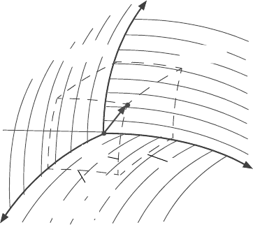
A point is obtained if we also fix ( ).
(3.6)
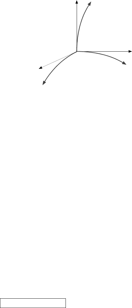
One may view this point as the origin of a local, in general non Cartesian
coordinate system (Fig. 3.1). Let us calculate the distance between this point
and the point . Using Cartesian
coordinates we have
.
(3.7)
Where of course
u
2
u
1
xyz,,()c
1
=
u
2
xyz,,()c
2
=
u
3
xxc
1
c
2
u
3
,,()=
yyc
1
c
2
u
3
,,()=
zzc
1
c
2
u
3
,,()=
u
3
u
3
c
3
=
u
1
xyz,,()c
1
=
u
2
xyz,,()c
2
=
u
3
xyz,,()c
3
=
Fig. 3.1
u
2
u
3
u
1
u
1
=
c
1
u
3
= c
3
u
2
=
c
2
P
P’
du
1
du
2
du
3
xxc
1
c
2
c
3
,,()=
yyc
1
c
2
c
3
,,()=
zzc
1
c
2
c
3
,,()=
P u
1
u
2
u
3
,,() P ' u
1
du
1
+ u
2
du
2
+ u
3
du
3
+,,()
ds
2
dx
2
dy
2
dz
2
++=
3.1 Coordinate Transformations 119
(3.8)
Substituting (3.8) into (3.7) and after ordering we obtain
(3.9)
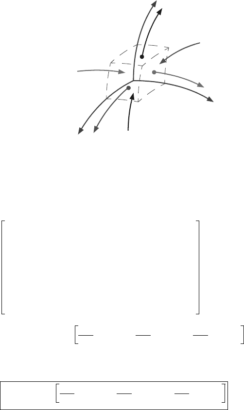
We will not use this rather inconvenient expression in its full generality, but restrict
ourselves to orthogonal coordinate systems. These are characterized by the fact that
the three coordinate lines in Fig. 3.1 are mutually perpendicular at every point. We
define the tangential vectors . For instance, the vector tangent to the line
, which was given in eq. (3.5) is determined by:
.
(3.10)
Similarly for the remaining vectors:
.
(3.11)
Fig. 3.2 shows the coordinate system of Fig. 3.1 with its tangent vectors.
dx
u
1
∂
∂ x
du
1
u
2
∂
∂ x
du
2
u
3
∂
∂ x
du
3
++=
dy
u
1
∂
∂ y
du
1
u
2
∂
∂ y
du
2
u
3
∂
∂ y
du
3
++=
dz
u
1
∂
∂z
du
1
u
2
∂
∂z
du
2
u
3
∂
∂ z
du
3
++=
ds
2
u
1
∂
∂ x
2
u
1
∂
∂ y
2
u
1
∂
∂ z
2
++ du
1
2
=
+
u
2
∂
∂ x
2
u
2
∂
∂y
2
u
2
∂
∂ z
2
++ du
2
2
+
u
3
∂
∂ x
2
u
3
∂
∂ y
2
u
3
∂
∂ z
2
++ du
3
2
+ 2
u
1
∂
∂x
u
2
∂
∂x
u
1
∂
∂y
u
2
∂
∂y
u
1
∂
∂z
u
2
∂
∂z
++ du
1
du
2
+
u
1
∂
∂x
u
3
∂
∂x
u
1
∂
∂y
u
3
∂
∂y
u
1
∂
∂z
u
3
∂
∂z
++ du
1
du
3
+
u
2
∂
∂x
u
3
∂
∂x
u
2
∂
∂y
u
3
∂
∂y
u
2
∂
∂z
u
3
∂
∂z
++ du
2
du
3
t
1
t
2
t
3
,,
u
3
t
3
u
3
∂
∂x
u
3
∂
∂y
u
3
∂
∂z
,,〈〉=
t
1
u
1
∂
∂x
u
1
∂
∂y
u
1
∂
∂z
,,〈〉=
t
2
u
2
∂
∂x
u
2
∂
∂y
u
2
∂
∂z
,,〈〉=
120 Formal Methods of Electrostatics
A coordinate system is orthogonal if the following holds for every point:
.
(3.12)
The vector from to is
.
(3.13)
Therefore the distance element (squared) is
.
(3.14)
This is a much shorter way to write eq. (3.9). For an orthogonal coordinate
system, because of eq. (3.12), the (square of the) distance element simplifies even
more
.
(3.15)
The only difference to the respective expression in Cartesian coordinates is the
occurrence of the scale factors which are spatially dependent, i.e., they are
generally different at differing positions in space. The volume element in
curvilinear coordinates is characterized by . Its edges are
, and thus has the volume element
.
(3.16)
Fig. 3.2
t
3
t
1
t
2
u
2
u
3
u
1
t
1
t
2
• 0=
t
2
t
3
• 0=
t
3
t
1
• 0=
PP'
drt
1
du
1
t
2
du
2
t
3
du
3
++=
ds
2
dr dr•=
t
1
2
du
1
2
t
2
2
du
2
2
t
3
2
du
3
2
++=
+ 2 t
1
t
2
• du
1
du
2
+ 2 t
1
t
3
• du
1
du
3
+ 2 t
2
t
3
• du
2
du
3
ds
2
t
1
2
du
1
2
t
2
2
du
2
2
t
3
2
du
3
2
++=
t
1
t
2
t
3
,,
du
1
du
2
du
3
,,
t
1
du
1
t
2
du
2
t
3
du
3
,,
dτ t
1
t
2
t
3
du
1
du
2
du
3
=
3.2 Vector Analysis for Curvilinear, Orthogonal Coordinate Systems 121
The infinitesimal line element or displacement has the components
(i=1,2,3)
(3.17)
and an infinitesimal area element has the components
(i, k ,l all different)
(3.18)
The factors are the diagonal elements of the so-called metric tensor, which has
off diagonal elements if the coordinate systems are not orthogonal.
3.2 Vector Analysis for Curvilinear, Orthogonal Coordinate
Systems
3.2.1 Gradient
Starting form the definition
and because of
one obtains
.
Similarly, for the other components
.
(3.19)
3.2.2 Divergence
The starting point for the definition of the divergence is the limit of a surface
integral of the type given by eq. (1.22). Using nomenclature established in Fig. 3.3,
one finds the vector a with its components a
1
, a
2
, a
3
ds
ds
i
t
i
du
i
=
dA
dA
i
t
k
t
l
du
k
du
l
=
t
i
2
∇ϕ()
u
1
ϕ u
1
∆u
1
u
2
u
3
,,+()ϕu
1
u
2
u
3
,,()–
∆s
1
-------------------------------------------------------------------------------------
∆u
1
0→
lim=
∆s
1
t
1
∆u
1
=
∇ϕ()
u
1
1
t
1
----
ϕ u
1
∆u
1
u
2
u
3
,,+()ϕu
1
u
2
u
3
,,()–
∆u
1
-------------------------------------------------------------------------------------
∆u
1
0→
lim=
1
t
1
----
u
1
∂
∂ϕ
=
∇ϕ
1
t
1
----
u
1
∂
∂ϕ 1
t
2
----
u
2
∂
∂ϕ 1
t
3
----
u
3
∂
∂ϕ
,,〈〉 =
a∇•
1
V
---
adA
∫
°
V 0→
lim=
122 Formal Methods of Electrostatics
,
i.e.,
.
(3.20)
3.2.3 Laplace Operator
Since
one may derive the Laplacian from both, eq. (3.19) and (3.20). One obtains
Fig. 3.3
u
2
u
3
u
1
a
3
(u
3
+du
3
)
a
3
(u
3
)
a
2
(u
2
+du
2
)
a
2
(u
2
)
a
1
(u
1
+du
1
)
a
1
(u
1
)
a∇•
1
t
1
t
2
t
3
du
1
du
2
du
3
-----------------------------------------
⋅⋅
du
1
du
2
du
3
0→
lim=
a
1
u
1
du
1
+()t
2
u
1
du
1
+()t
3
u
1
du
1
+()du
2
du
3
a
1
u
1
()t
2
u
1
()t
3
u
1
()du
2
du
3
–
+ a
2
u
2
du
2
+()t
1
u
2
du
2
+()t
3
u
2
du
2
+()du
1
du
3
a
2
u
2
()t
1
u
2
()t
3
u
2
()du
1
du
3
–
+ a
3
u
3
du
3
+()t
1
u
3
du
3
+()t
2
u
3
du
3
+()du
1
du
2
a
3
u
3
()t
1
u
3
()t
2
u
3
()du
1
du
2
–
u
1
∂
∂
a
1
t
2
t
3
()
u
2
∂
∂
a
2
t
1
t
3
()
u
3
∂
∂
a
3
t
1
t
2
()++ du
1
du
2
du
3
t
1
t
2
t
3
du
1
du
2
du
3
-------------------------------------------------------------------------------------------------------------------------------------
du
1
du
2
du
3
0→
lim=
a∇•
1
t
1
t
2
t
3
-------------
u
1
∂
∂
a
1
t
2
t
3
()
u
2
∂
∂
a
2
t
1
t
3
()
u
3
∂
∂
a
3
t
1
t
2
()++=
∆ϕ ∇ϕ∇• ∇
2
ϕ==
3.2 Vector Analysis for Curvilinear, Orthogonal Coordinate Systems 123
.
(3.21)
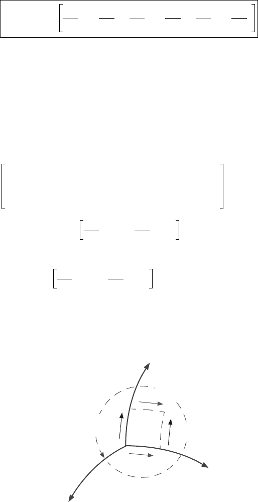
3.2.4 Circulation
To calculate the curl, we start from eq. (1.34) and use the right hand rule to
establish the relation between the direction of the circulation (also called the
rotation) and the direction of the line integral of Section 1.7. Using the notation
from Fig. 3.4, one finds:
.
The other two components of are derived in the same way. The end result is
∇
2
ϕ
1
t
1
t
2
t
3
-------------
u
1
∂
∂
t
2
t
3
t
1
--------
u
1
∂
∂ϕ
u
2
∂
∂
t
1
t
3
t
2
--------
u
2
∂
∂ϕ
u
3
∂
∂
t
1
t
2
t
3
--------
u
3
∂
∂ϕ
++=
Fig. 3.4
u
2
u
3
u
1
a
2
(u
3
)
direction of
path
a
3
(u
2
+du
2
)
a
3
(u
2
)
a
2
(u
3
+du
3
)
a∇×()
u
1
1
t
2
t
3
du
2
du
3
---------------------------
⋅
du
2
du
3
0→
lim=
a
2
u
3
()t
2
u
3
()du
2
⋅ a
3
u
2
du
2
+()t
3
u
2
du
2
+()du
3
⋅+
a–
2
u
3
du
3
+()t
2
u
3
du
3
+()du
2
⋅
a–
3
u
2
()t
3
u
2
()du
3
⋅
u
2
∂
∂
a
3
t
3
()
u
3
∂
∂
a
2
t
2
()– du
2
du
3
t
2
t
3
du
2
du
3
------------------------------------------------------------------------------
du
2
du
3
0→
lim=
1
t
2
t
3
--------
u
2
∂
∂
a
3
t
3
()
u
3
∂
∂
a
2
t
2
()–=
a∇×