Lehner G. Electromagnetic Field Theory for Engineers and Physicists

Подождите немного. Документ загружается.

124 Formal Methods of Electrostatics

(3.22)

Using the unit vectors of a coordinate system,

we may also write curl a in its determinant form

(3.23)

(3.24)

3.3 Some Important Coordinate Systems

Of the many interesting coordinate systems, this book will only employ three:

Cartesian, cylindrical, and spherical coordinates. We will summarize the results of

our previous discussion for these coordinate systems.

a∇×

--------

∂

()

∂

()–

--------

∂

()

∂

()–

--------

∂

()

∂

()–

----=

a∇×

--------

∂

a∇×

-------------

∂

3.3 Some Important Coordinate Systems 125

3.3.1 Cartesian Coordinates

For Cartesian coordinates, the scale factors are, of course, and

from eq. (3.19) through eq. (3.24), we obtain the familiar expressions

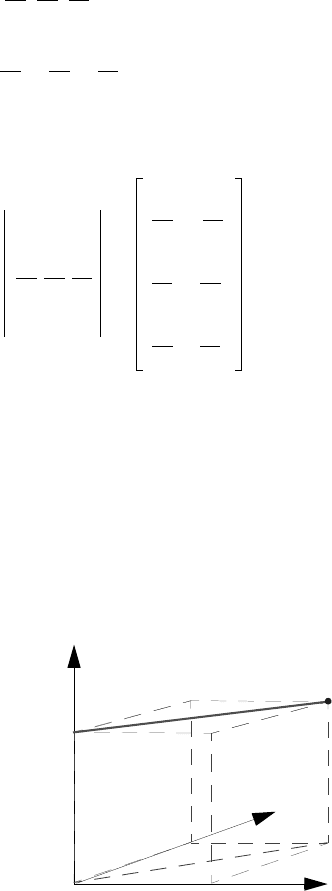
3.3.2 Cylindrical Coordinates

The case of cylindrical coordinates is illustrated in Fig. 3.5. The coordinates are

(3.25)

1===

∇ϕ

x∂

∂ϕ

y∂

∂ϕ

z∂

∂ϕ

,,〈〉=

a∇•

x∂

∂a

y∂

∂a

z∂

∂a

++=

∇

∂

∂x

---------

∂

∂y

---------

∂

∂z

---------++=

a∇×

x∂

∂

y∂

∂

z∂

∂

y∂

∂a

z∂

∂a

–

z∂

∂a

x∂

∂a

–

x∂

∂a

y∂

∂a

–

Fig. 3.5

ϕ=











126 Formal Methods of Electrostatics

or expressed in Cartesian coordinates

(3.26)

With this, eq. (3.10), and (3.11) it follows for the tangent vectors in Cartesian

coordinates:

(3.27)

i.e.,

(3.28)

and consequently for the volume element and the (squared) distance element

(3.29)

, (3.30)

and furthermore

(3.31)

. (3.32)

. (3.33)

(3.34)

Be careful not to confuse the angle with the potential , which was up to now

also labeled with . We will identify the potential with some other symbol

wherever confusion with the angle is anticipated.

xrϕcos=

yrϕsin=

zz=











ϕcos ϕsin 0,,〈〉=

r ϕsin– r ϕcos 0,,〈〉=

001,,〈〉=











1= 









dτ rdrdϕdz=

dϕ

++=

∇φ

r∂

∂

---

ϕ∂

∂

z∂

∂

,,〈〉φ=

a∇•

---

r∂

∂

---

ϕ∂

∂

z∂

∂

++=

∇

---

r∂

∂

r∂

∂ 1

-----

∂

∂ϕ

---------

∂

∂z

--------++





φ=

a∇×

a∇×()

---

ϕ∂

∂

z∂

∂

–

z∂

∂

r∂

∂

–

---

r∂

∂

()

---

ϕ∂

∂

–

ϕφ

3.3 Some Important Coordinate Systems 127

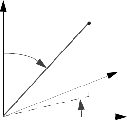
3.3.3 Spherical Coordinates

Fig. 3.6 illustrates the spherical coordinate system.

The spherical coordinates are,

(3.35)

or expressed in terms of the Cartesian coordinates

(3.36)

For the tangent vectors

(3.37)

and

(3.38)

and consequently for the volume element and (squared) distance element

(3.39)

, (3.40)

Fig. 3.6

θ=

ϕ=











xrθsin ϕcos=

yrθsin ϕsin=

zrθcos=











θsin ϕcos θsin ϕsin θcos,,〈〉=

r θcos ϕcos r θcos ϕsin r θsin–,,〈〉=

r θsin ϕsin– r θsin ϕcos–0,,〈〉=











θsin











dτ r

θsin drdθdϕ=

dθ

θsin

dϕ

++=

128 Formal Methods of Electrostatics

and

(3.41)

, (3.42)

, (3.43)

(3.44)

3.4 Some Properties of Poisson’s and Laplace’s Equations

(Potential Theory)

Poisson’s and Laplace’s equation (2.11) and (2.12), respectively are the basis for

the formal treatment of electrostatics.

3.4.1 Problem Description

A large class of electrostatic problems are described in the following way:

Consider an arbitrarily shaped region, with an arbitrary distribution of volume

charges inside. Given is the potential on its boundary or the perpendicular

component of the electric field on the boundary, i.e., . This

represents Neumann’s boundary value problem when is prescribed. On the

other hand, when is prescribed, it is called Dirichlet’s boundary value problem.

Of course, it is possible to prescribe on part of the boundary and on the

other part, in which case one is dealing with a mixed boundary value problem.

The region in question may be bounded by any number of arbitrarily shaped

surface areas.

One can uniquely solve these kind of boundary value problems using the

methods of potential theory . Its proof involves Green’s integral theorems.

3.4.2 Green’s Theorems

The starting point is Gauss’ integral theorem

∇φ

r∂

∂

---

θ∂

∂

r θsin

-------------

ϕ∂

∂

,,〈〉φ=

a∇•

-----

r∂

∂

r θsin

-------------

θ∂

∂

θsin a

r θsin

-------------

ϕ∂

∂

++=

∇

-----

r∂

∂

r∂

∂ 1

θsin

----------------

θ∂

∂

θ∂

∂

sin

θsin

------------------

∂

∂ϕ

---------





φ=

a∇×

a∇×()

r θsin

-------------

θ∂

∂

θsin a

r θsin

-------------

ϕ∂

∂

–

r θsin

-------------

ϕ∂

∂

---

r∂

∂

–

---

r∂

∂

()

---

θ∂

∂

–

ρ r() ϕ

∇ϕ()

∂ϕ ∂n⁄=

∂ϕ ∂n⁄

ϕ∂ϕ∂n⁄

3.4 Some Properties of Poisson’s and Laplace’s Equations 129

Define a vector a as

where and are arbitrary scalar functions. When substituting, one obtains

(3.45)

This is Green’s first identity. It is permissible to exchange and , as they

are arbitrary anyway. This gives

(3.46)

Now we use:

and ,

as well as

and similarly

Using these relations and subtracting (3.46) from (3.45) yields Green’s second

identity, also known as Green’s theorem.

(3.47)

On the other hand, if we let in one of the two equations (3.46) or (3.45),

then we obtain one of Green’s integral theorems:

(3.48)

If the functions and depend on two variables only, then (3.47) and (3.48)

reduce even more:

and

a∇• τd

∫

a dA•

∫

a ψ∇φ=

ψφ

a∇• τd

∫

ψ∇φ()∇• τd

∫

ψ∇φ∇•()∇ψ()∇φ()•+[]τd

∫

ψ∇φ dA•

∫

ψφ

φ∇ψ()∇• τd

∫

φ∇ψ∇•()∇φ()∇ψ()•+[]τd

∫

φ∇ψ dA•

∫

∇φ()∇• ∇

φ= ∇ψ()∇• ∇

ψ=

∇ψ dA•∇ψndA•∇ψ()

dA==

n∂

∂ψ

dA ,=

∇φ dA•

n∂

∂φ

dA=

ψ∇

φφ∇

ψ–()τd

∫

n∂

∂φ

n∂

∂ψ

–





∫

φψ=

φ∇

φ∇φ()

+()τd

∫

n∂

∂φ





∫

φψ

ψ∇

φφ∇

ψ–()Ad

∫

n∂

∂φ

n∂

∂ψ

–





∫

φ∇

φ∇φ()

+()Ad

∫

n∂

∂φ





∫

130 Formal Methods of Electrostatics

For the one dimensional case this gives

and

These are simple integrations by parts. Green’s integral theorems are thus simply

generalizations of integrations by parts to two or three dimensions, respectively.

3.4.3 Proof of Uniqueness

Suppose (for our Neumann, Dirichlet, or mixed problem) there are two solutions

and . This means that

and the boundary conditions shall also be satisfied.

We define a new function as the difference

then

which means that it has to satisfy Laplace’s equation. Furthermore, the potential

along the boundary is

or – in case of mixed problems – one of the equations along part of the boundary

and the other equation along the remainder of the boundary. We apply Green’s

theorem in its form (3.48) to and obtain

Since is always positive, this can only be true if the integrand is identically

zero

ψφ'' φψ''–()xd

∫

ψφ' φψ'–[]

φφ'' φ'

+()xd

∫

φφ'[]

∇

ρ r()

----------–=

∇

ρ r()

----------–=

–=

∇

–0==

n∂

∂

∇ϕ

()

τd

∫

∇ϕ

()

∇ϕ

131

The case of a Dirichlet, or even the mixed boundary value problem requires

that everywhere. For Neumann’s problem, is determined, except for a

physically insignificant constant.

The problem may also be posed in a different way. Given is the charge of a

conductor in an electric field. Then

(The negative sign in is due to the fact that the normal component

points outwardly, relative to the region that contains the field, which means it

points into the conductor). Therefore

Thus, it is not that is prescribed along the boundary but the integral

. Furthermore, is constant on the surface, although its value is yet

unknown. If we now have two solutions and , then, as before, Laplace’s

equation applies to both, and to their difference. Integrating both solutions over the

boundary gives

Therefore

as before. Again we find

and

These uniqueness proofs have a common theme, and are formally based on eq.

(3.48), which concludes that if the boundary conditions require on the

surface, together with , that then has to vanish everywhere. There is a

plausible way to understand this. One can prove that in an area where ,

may neither have a maximum nor a minimum. If there were a maximum (or a

minimum) of at any point inside the region, then in a neighborhood of this point,

all lines of had to point towards (or away from) it. Any surface in the vicinity

const=

n∂

∂ϕ

–

-----==

σε

⁄–=

Q σ Ad

∫

n∂

∂ϕ

∫

∂ϕ dn⁄

∂ϕ dn⁄()Ad

∫

Q ε

n∂

∂ϕ

∫

n∂

∂ϕ

∫

∇ϕ

()

τd

∫

n∂

∂

∫

–()

∂ϕ

–()

∂n

-------------------------

∫

–()

∂ϕ

–()

∂n

--------------------------

∫

–()

QQ–

--------------





0==

∇ϕ

const=

∇

ϕ 0=

ϕ 0= ϕ

∇

ϕ 0=

∇ϕ

3.4 Some Properties of Poisson’s and Laplace’s Equations

132 Formal Methods of Electrostatics

of the maximum (or minimum) would be penetrated by a non-vanishing electrical

flux. This is only possible if there are volume charges present, which would require

. Therefore, the assumption of a maximum or minimum inside of this area

would lead to a contradiction. Then, if on the boundary, it can not be larger

inside, but it can also not be smaller than zero inside and consequently

everywhere in the region. In other words: If in a region , then the

function may have its maximum or minimum values only on the boundary of that

region. Uniqueness of the solution of Dirichlet’s boundary value problem is an

immediate consequence of this statement.

3.4.4 Models

The equation has a frequent occurrence in physical science and it

describes a vast number of problems. This enables one to frequently map physical

problems onto a corresponding electrostatic problem. For example, the two-

dimensional Laplace’s equation

also describes the displacement of a membrane suspended on a frame which is

considered to be small. The boundary (frame) defines and inside .

Such a membrane can be considered a model for electrostatic problems.

3.4.5 Dirac’s Delta Function (δ-Function)

The -function is particularly useful in the following, which is why we will

introduce it here. It shall be noted that our exposition here does not substitute a

rigorous mathematical introduction.

A rough, illustrative way to describe the character of the -function is to note

that it vanishes everywhere except for one particular point of its argument (namely

0), where it takes an infinite value, exactly such that its integral equals 1.

(3.49)

(3.50)

The -function is not a function in the usual sense. It belongs to a more general

category of functions, which sometimes are called improper functions, generalized

functions, or distributions. Another possibility is to imagine the -function as the

limit of a series of functions. It can be constructed in various ways, for example,

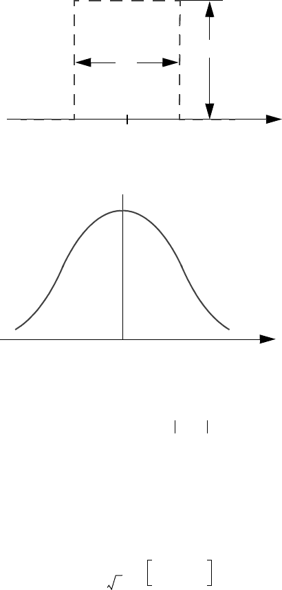
1. The limit of a series of rectangular functions as illustrated in Fig. 3.7.

Thus

∇

ϕ 0≠

ϕ 0=

∇

ϕ 0=

∇

ϕ 0=

∂





ϕ 0=

ϕ∇

ϕ 0=

δ xx'–()

0 forxx'≠

∞ for xx'=







δ xx'–()xd

∞–

+∞

∫

133

and

2. The limit of a series of Gaussian functions as illustrated in Fig. 3.8. Now

where

and

Fig. 3.7

x=x’

1/h

x()

h for xx'–

------

≤

0else











δ xx'–() g

x()

h ∞→

lim=

Fig. 3.8

x=x’

x()

a π

----------

xx'–()

-------------------–exp=

x()xd

∞–

+∞

∫

3.4 Some Properties of Poisson’s and Laplace’s Equations