Lehner G. Electromagnetic Field Theory for Engineers and Physicists

334 Basics of Magnetostatics

.

(5.201)

One can show that the integral is positive. Therefore, is positive when ,

and is negative when (assuming a positive current I). The former case

results in attracting forces and the latter in repelling ones.

If the current loop (in region 1) is in vacuum ( ), then it is attracted by a

paramagnetic cylinder, and repelled from a diamagnetic one. This is true also for

differently shaped bodies and current loops. The total magnetization current is

.

According to eqs. (3.178) through (3.180), this limit is and therefore

.

(5.202)

The case when an external field shall be shielded by a cylinder with infinite

conductivity can formally be described by letting . With one

obtains

k

ϕ

z()

µ

2

µ

1

–()Ir

0

πµ

0

r

1

------------------------------

K

1

kr

0

()I

0

kr

1

() kz()cos

K

1

kr

1

()I

0

kr

1

()

µ

2

µ

1

------

K

0

kr

1

()I

1

kr

1

()+

-----------------------------------------------------------------------------------------

kd

0

∞

∫

=

k

ϕ

µ

2

µ

1

>

µ

2

µ

1

<

µ

1

µ

0

=

k

ϕ

z()kd

∞–

+∞

∫

µ

2

µ

1

–()Ir

0

πµ

0

r

1

------------------------------

K

1

kr

0

()I

0

kr

1

() kz()cos zd

∞–

+

∞

∫

K

1

kr

1

()I

0

kr

1

()

µ

2

µ

1

------

K

0

kr

1

()I

1

kr

1

()+

-----------------------------------------------------------------------------------------

kd

0

∞

∫

=

k

ϕ

z()kd

∞–

+∞

∫

µ

2

µ

1

–()Ir

0

πµ

0

r

1

------------------------------

K

1

kr

0

()I

0

kr

1

()2πδ k()

K

1

kr

1

()I

0

kr

1

()

µ

2

µ

1

------

K

0

kr

1

()I

1

kr

1

()+

-----------------------------------------------------------------------------------------

kd

0

∞

∫

=

k

ϕ

z()kd

∞–

+∞

∫

µ

2

µ

1

–()Ir

0

µ

0

r

1

------------------------------

K

1

kr

0

()I

0

kr

1

()

K

1

kr

1

()I

0

kr

1

()

µ

2

µ

1

------

K

0

kr

1

()I

1

kr

1

()+

-----------------------------------------------------------------------------------------

k 0→

lim=

Fig. 5.65 Mag-

r

1

r

0

⁄

k

ϕ

z()kd

∞–

+∞

∫

µ

2

µ

1

–()I

µ

0

-------------------------=

µ

2

0= µ

1

µ

0

=

5.12 Magnetic Energy, Magnetic Flux and Inductance Coefficients 335

(5.203)

and the total current is

.

(5.204)

The entire surface current in this case totals to exactly -I, i.e., the same amount as

the current in the loop, anti-parallel, however. This is necessary. Otherwise, there

had to be a magnetic field in the cylinder due to Ampere’s law.

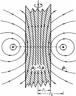
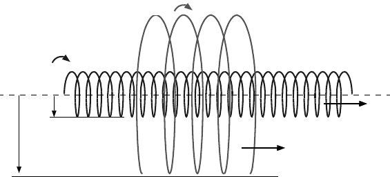
Fig. 5.65 provides an example for the field lines when .

5.12 Magnetic Energy, Magnetic Flux and Inductance

Coefficients

5.12.1 Magnetic Energy

We have discovered already in Sect. 2.14.1 that the potential energy density stored

in a magnetic field is . The total energy is therefore

.

Using (5.7) yields

.

With the vector identify

this gives

or

.

The surface integral has to include all possible boundaries. A sphere at infinity

does not provide any contributions because of the sufficiently fast decrease of

as R increases (the product is proportional to ). This can be seen from

eqs. (5.16) and (5.17). Inside surfaces – they need to be considered from both sides

– do not provide any contribution as long as is continuous. As we

will see shortly, this is the case, as long as there are no surface currents in the

boundary. The energy is then:

.

(5.205)

k

ϕ

z()

Ir

0

πr

1

--------

K

1

kr

0

()

K

1

kr

1

()

-------------------

kz()cos kd

0

∞

∫

–=

k

ϕ

z()zd

∞–

+∞

∫

I–=

µ

2

5µ

1

=

12⁄()µH

2

12⁄()HB•=

W

1

2

---

HB•τd

V

∫

=

W

1

2

---

HA∇×()•τd

V

∫

=

AH×()∇• HA∇×()• AH∇×()•–=

W

1

2

---

AH×()∇• τd

V

∫

1

2

---

AH∇×()•τd

V

∫

+=

W

1

2

---

AH×()da•

∫

°

1

2

---

AH∇×()•τd

V

∫

+=

AH× R

3–

AH×()da•

W

1

2

---

Ag•τd

V

∫

=

336 Basics of Magnetostatics

This interesting result should be compared to a similar equation obtained for the

electrostatic energy (2.171):

.

If there are surface currents in the boundary, then the surface integral contributes to

the energy, namely

By eq. (5.96), this gives

.

These contributions, originating from surface currents, can be thought of as being

contained in eq. (5.205). Now we have to consider all currents in this equation,

even surface currents, for which, indeed, is infinitely large, but remains

finite.

By (5.16) and (5.205) it is finally:

.

(5.206)

Now consider a system consisting of n closed conductors with the currents ,

. Then

,

and

i.e.,

,

(5.207)

having defined the so-called inductance coefficients in the following way

.

(5.208)

W

1

2

---

ρϕdτ

V

∫

=

W

a

1

2

---

AH×()da•

∫

°

1

2

---

AH

2

H

1

–()×[]n

2

• a

i

d

a

i

∫

i

∑

==

1

2

---

AH

2

H

1

–()n

2

×[]• a

i

.d

a

i

∫

i

∑

=

W

a

1

2

---

Ak• a

i

d

a

i

∫

i

∑

=

ggdτ

W

µ

0

8π

------

gr() gr'()•τd τ'd

rr'–

-----------------------------------------

V'

∫

V

∫

=

g

i

r()

i 12… n,, ,=()

gr() g

i

r()

i 1=

n

∑

=

W

µ

0

8π

------

g

i

r() g

j

r'()•τd τ'd

rr'–

--------------------------------------------

V'

∫

V

∫

ij, 1=

n

∑

=

µ

0

8π

------

I

i

I

j

g

i

r() g

j

r'()•τd τ'd

I

i

I

j

rr'–

--------------------------------------------

.

V'

∫

V

∫

i

j,

1=

n

∑

=

W

1

2

---

L

ij

I

i

I

j

ij, 1=

n

∑

=

L

ij

L

ij

µ

0

4πI

i

I

j

--------------

g

i

r() g

j

r'()•τd τ'd

rr'–

--------------------------------------------

V'

∫

V

∫

=

5.12 Magnetic Energy, Magnetic Flux and Inductance Coefficients 337

The reciprocity (symmetry) of these coefficients

(5.209)

is an immediate consequence of definition (5.208). When , these coefficients

are called self-inductance coefficients.

There are two ways to calculate : either use (5.208) or calculate W and then

compare it with (5.207). The latter is usually the more convenient approach. Two

simple examples shall serve to illustrate this.

1) The Coaxial Cable (Fig. 5.66)

If the conductors in the cable are very thin (or they have infinite conductivity), then

the situation is as sketched in Fig. 5.66. The field is

.

Total energy becomes infinite if the length is infinite. Per unit length, however, it

remains finite.

which yields the self-inductance coefficients per unit length

L

ij

L

ji

=

ij=

L

i

j

Fig. 5.66 Coaxial Cable

g

z

r()

z

r

a

b

a

b

rr

B

ϕ

r()

a b

B

ϕ

r()

µ

0

I

2πr

---------=

H

ϕ

r()

I

2πr

---------=

1

2

---

BH•

µ

0

I

2

8π

2

r

2

--------------=

W

l

-----

µ

0

8π

2

---------

I

2

r

2

-----

2πrrd

a

b

∫

µ

0

I

2

4π

-----------

rd

r

-----

a

b

∫

==

µ

0

I

2

4π

-----------

b

a

---ln

1

l

---

1

2

---

L

11

I

2

,==

338 Basics of Magnetostatics

,

(5.210)

a frequently used, and in practice important result.

2) Two infinitely long Coils (Fig. 5.67)

Consider the currents and flowing in the two coils with and turns per

unit length, respectively. Inside coil 1, this creates the field

and between coil 2 and coil 1 the field

.

Then

and by comparing coefficients

L

l

---

L

11

l

--------

µ

0

2π

------

b

a

---ln==

Fig. 5.67 Two infinitely long Coils

I

1

I

2

n

2

I

2

n

1

I

1

r

1

r

2

H

I2

H

I1

I

1

I

2

n

1

n

2

H

z1

n

1

I

1

n

2

I

2

+=

H

z2

n

2

I

2

=

W

l

-----

µ

0

n

1

I

1

n

2

I

2

+()

2

-----------------------------------------

r

1

2

π

µ

0

n

2

I

2

()

2

------------------------

r

2

r

1

2

–()π+=

µ

0

π

2

---------

n

1

2

I

1

2

r

1

2

2n

1

n

2

I

1

I

2

r

1

2

n

2

I

2

r

2

++[]=

1

2

---

L

11

l

--------

I

1

2

1

2

---

L

12

l

--------

I

1

I

2

1

2

---

L

21

l

--------

I

1

I

2

1

2

---

L

22

l

--------

I

2

+++=

1

2

---

L

11

l

--------

I

1

2

L

12

l

--------

I

1

I

2

1

2

---

L

22

l

--------

I

2

++=

5.12 Magnetic Energy, Magnetic Flux and Inductance Coefficients 339

.

(5.211)

Notice that the currents carry a sign and the mixed terms (here )

may be both, positive or negative.

5.12.2 Magnetic Flux

Consider one or more circuits with the magnetic energy

.

In the outside space, i.e., outside the current carrying conductor, the field may be

written by means of the scalar potential

.

We now assume that with respect to the extent of the outside space, the width of the

conductor is negligible. Consequently, we only need to take the volume integral

over the outside space and the inside contribution, including that of the magnetic

energy inside is negligible. This gives

.

Because of the vector identity

this becomes

.

Using

and applying Gauss’ integral theorem gives

.

If we initially concentrate on one conductor (shown in Fig. 5.68) we get

1

l

---

L

11

µ

0

πr

1

2

n

1

2

=

1

l

---

L

12

1

l

---

L

21

µ

0

πr

1

2

n

1

n

2

==

1

l

---

L

22

µ

0

πr

2

n

2

=











I

12,

I

1

I

2

∼

W

µ

0

2

------

H

2

τd

V

∫

=

ψ

H ψ∇–=

W

µ

0

2

------

ψ∇()

2

τd

V

∫

=

ψψ∇()∇• ψ∇

2

ψψ∇()

2

+=

W

µ

0

2

------

ψψ∇()∇• ψ∇

2

ψ–[]τd

V

∫

=

∇

2

ψ 0=

W

µ

0

2

------

ψψ∇[]Ad•

A

∫

=

340 Basics of Magnetostatics

Because

is continuous, that is,

and therefore the energy becomes

.

By (5.58) and in analogy to the electrostatic dipole layer (see Sect. 2.5.3),

is constant along the entire separating surface

.

This makes

,

(5.212)

having used the fact that

is the flux through the separating surface. On the other hand, since

Fig. 5.68

n

1

I

2

1

n

2

surface at infinity

A

∞

separating surface

A

s

W

µ

0

2

------

ψψ∇[]Ad•

A

∞

∫

µ

0

2

------

ψψ∇[]Ad•

A

s

∫

+=

0

µ

0

2

------

ψψ∇[]Ad•

A

s

∫

+=

µ

0

2

------

ψ

1

x∂

∂ψ





1n

ψ

2

x∂

∂ψ





2n

– A

1

.d•

A

s

∫

=

µ

0

x∂

∂ψ

B

n

–=

µ

0

x∂

∂ψ





1n

µ

0

x∂

∂ψ





2n

µ

0

x∂

∂ψ





n

B

n

–===

W

µ

0

2

------

ψ

1

ψ

2

–()

x∂

∂ψ





n

A

1

d

A

s

∫

1

2

---

ψ

2

ψ

1

–()B

n

A

1

d

A

s

∫

==

ψ

2

ψ

1

–

ψ

2

ψ

1

– I=

W

1

2

---

Iφ=

B

n

Ad

A

s

∫

φ=

5.12 Magnetic Energy, Magnetic Flux and Inductance Coefficients 341

,

comparison shows that consequently

.

(5.213)

This result may be generalized to arbitrarily many conductors:

.

(5.214)

Conversely, because of

,

it is also

.

(5.215)

One concludes that the flux through a conductor loop is a linear function of all

currents

If the currents are time dependent, then the magnetic flux is also time dependent.

The law of electromagnetic induction states, except for the sign, that the temporal

change of equals the EMF induced in the conductor loop. That is the

reason why the inductance coefficients are important for the induced voltages in a

network, which also explains their name.

Eq. (5.215) provides another avenue to calculate the inductance coefficients.

Consider for example, the two coils calculated above. For these one has:

,

which, in accordance with (5.211) gives

W

1

2

---

L

11

I

2

1

2

---

L

11

I()I==

φ L

11

I=

W

1

2

---

I

i

φ

i

i 1=

n

∑

=

W

1

2

---

L

ij

I

i

I

j

ij, 1=

n

∑

1

2

---

I

i

i 1=

n

∑

L

ij

I

j

j 1=

n

∑

==

φ

i

L

ij

I

j

j 1=

n

∑

=

φ

1

L

11

I

1

L

12

I

2

L

13

I

3

…+++=

φ

2

L

21

I

1

L

22

I

2

L

23

I

3

…+++=

………………………………

∂φ

i

∂t⁄

1

l

---

φ

1

n

1

r

1

2

πµ

0

n

1

I

1

r

1

2

πµ

0

n

2

I

2

+()=

1

l

---

φ

2

n

2

r

1

2

πµ

0

n

1

I

1

r

2

πµ

0

n

2

I

2

+()=

342 Basics of Magnetostatics

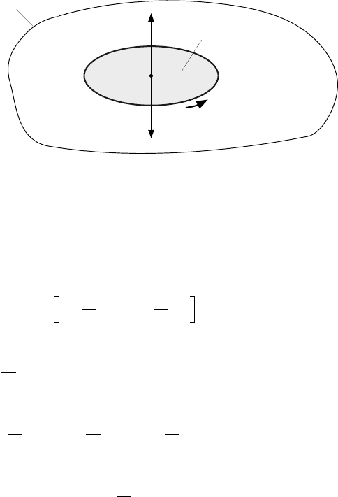
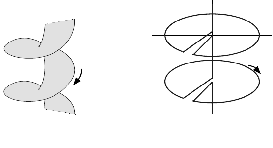
The fact that is proportional to shall be explained more plausibly. One

factor is a result of the magnetic inductance by the number of turns per unit

length. The second factor results from the surface, shown in Fig. 5.69, that

borders the coil and which connects the individual turns in a helical way. The

projection of this surface onto a plane perpendicular to the coil’s axis gives the

multiple of the coil’s cross section. Fig. 5.70 gives a schematic representation of

this.

Fig. 5.70

I

1

I

1

Fig. 5.69

1

l

---

L

11

µ

0

πr

1

2

n

1

2

=

1

l

---

L

12

1

l

---

L

21

µ

0

πr

1

2

n

1

n

2

==

1

l

---

L

22

µ

0

πr

2

n

2

.=

L

11

n

1

2

n

1

n

1

n

1

6 Time Dependent Problems I (Quasi Stationary

Approximation)

Maxwell’s equations were introduced in Chapter 1, but with a few exceptions, we

have not discussed them in their complete form. So far, we have focused on time

independent problems, specifically electrostatics in Chapter 2 and 3, stationary

electric currents in Chapter 4 and magnetostatics in Chapter 5. Now, we turn to

time dependent problems. We will do this in two steps. The time dependent

Maxwell equations differ from the stationary ones by two terms, the displacement

current in the first and the magnetic induction in the second

Maxwell equation. We will account for this fact in our proceedings. Specifically,

the displacement current may be neglected in a first approximation, while the law

of induction needs to be considered. This approximation does not allow us to

describe electromagnetic waves, since the displacement current is vital for these.

On the other hand, skin effect, eddy currents, and similar effects can be described

without the displacement current term. The applicability of this so-called quasi

stationary approximation is limited to cases where the temporal changes do not

occur too rapidly. We will postpone the discussion of the complete version of

Maxwell’s equations to the next chapter, (Chapter 7), where we will study

electromagnetic waves by including the displacement current term.

6.1 Faraday’s Law of Magnetic Induction

6.1.1 Induction by a Temporal Change of B

Consider a time dependent magnetic field described by the magnetic induction or

also called the magnetic flux density and a contour C, fixed in space. The

contour may be implemented by an infinitely thin, conducting material. If A is the

area that C circumscribes, then by our definition, eq. (1.66), the magnetic flux

penetrating this area is

.

(6.1)

The time dependent magnetic field induces an electric field , which

can be described using eq. (1.68)

.

(6.2)

The line integral of the electric field is given by the time derivative of the magnetic

flux:

.

(6.3)

Expressed in a different form, one writes

∂D ∂t⁄∂B ∂t⁄

Brt,()

φ Brt,()Ad•

A

∫

=

Brt,() Ert,()

Ert,()∇×

t∂

∂

Brt,()–=

Esd•

C

∫

°

E∇×()Ad•

A

∫

∂B

∂t

-------

Ad

A

∫

–

t∂

∂

BAd•

A

∫

–

t∂

∂φ

–====

G. Lehner, Electromagnetic Field Theory for Engineers and Physicists,

Lehner G. Electromagnetic Field Theory for Engineers and Physicists

Подождите немного. Документ загружается.