Lehner G. Electromagnetic Field Theory for Engineers and Physicists

Подождите немного. Документ загружается.

364 Time Dependent Problems I (Quasi Stationary Approximation)

(6.60)

This requires to find all singularities and their residues. The Laurent series (6.57)

shows that a residue of for a pole of order 1 can be written as

(6.61)

For a pole of order m, the Laurent series tells us that

(6.62)

In case of an essential singularity, i.e., when m is infinitely large, then

eq. (6.62) does not help. In this case we have to go back to the Laurent series itself.

Frequently, if , but or , then l’Hospital’s

rule

(6.63)

is a useful tool to determine the necessary limits to find the residues according to

(6.61) and (6.62). However, if and , then the procedure may

be repeated:

(6.64)

etc.

6.4 Field Diffusion in the Two-sided Infinite Space

We will investigate the behavior of a magnetic field in a uniformly

conductive material ( ). It satisfies the diffusion equation

(6.65)

Using the dimensionless time

(6.66)

and the dimensionless spatial coordinate

(6.67)

where as before, is an arbitrary length, then

(6.68)

A solution to this equation is for example,

ft() sum of all residues of f

p() pt()exp[]

∑

z()

1–

fz()zz

–()

→

lim=

1–

m 1–()!

--------------------

m 1–

----------------

fz()zz

–()

[]

→

lim=

fa() ga() 0== g' a() 0≠ f ' a() 0≠

fx()

gx()

----------

xa→

lim

f ' a()

g' a()

------------=

g' a() 0=

' a() 0=

fx()

gx()

----------

xa→

lim

f ' x()

g' x()

-----------

xa→

lim

f '' x()

g'' x()

-------------==

xt,()

κµ,

∂

B xt,() µκ

t∂

∂

xt,()=

----

µκl

-----------==

--=

∂

ξτ,()

τ∂

∂

ξτ,()=

6.4 Field Diffusion in the Two-sided Infinite Space 365

(6.69)

which can easily be verified by substitution. The solution also makes physically

sense because it remains finite for both , as well as for (it

vanishes). This is a Gaussian curve. Its width depends on the elapsed time, more

precisely, it widens for increasing times. For small times, the curve is narrow and

very high. Its integral from to is constant ( ) for all times

(6.70)

Disregarding the factor , for this expresses a δ-function, which can be

defined as the limit of a Gaussian curve (see Sect. 3.4.5):

(6.71)

and therefore

(6.72)

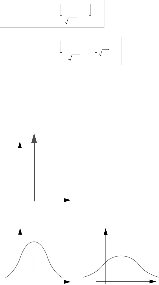
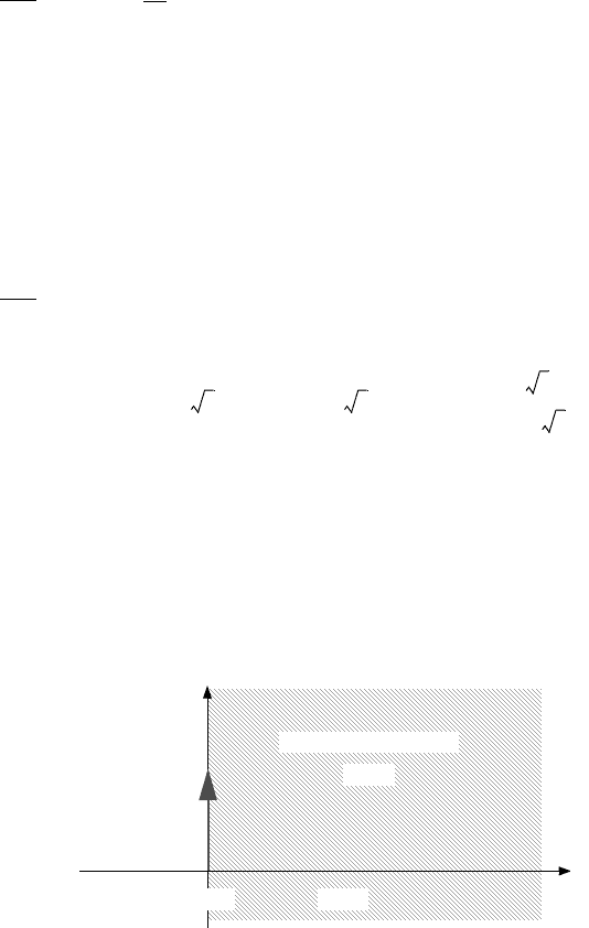
Consequently, according to (6.69), is the solution to the diffusion problem

in the infinite space with the initial condition given by (6.72). The initially closely

localized field flows gradually more and more apart (Fig. 6.17). From a formal

perspective, this behavior is entirely analogous to the theory of heat conductivity.

The special solution given here gives us – and this makes it so significant – the

solution to much more general problems. If the initial field is given in an arbitrary

shape

(6.73)

then we can find its solution by the superposition of many δ-functions:

(6.74)

That is, the initial field consists of pieces of the form

(6.75)

The contribution of such a piece at a later time is

(6.76)

The overall field results when superposing all the contributions, i.e., the integral

ξτ,()B

ξξ'–()

4τ

--------------------

–exp

4πτ

----------------------------------------

ξ∞–→ξ+∞→

ξ∞–→ξ+∞→ B

4πτ

-------------

ξξ'–()

4τ

--------------------

–exp ξd

∞–

+∞

∫

τ 0→

ξξ'–()

4τ

--------------------

–exp

4πτ

----------------------------------------

τ 0→

lim δξ ξ'–()=

ξ 0,()B

δξ ξ'–()=

ξτ,()

ξ 0,()h ξ()=

ξ 0,()h ξ() h ξ

()δξξ

–()ξ

∞–

+∞

∫

ξ 0,()δξξ

–()h ξ

()ξ

ξτ,()h ξ

()

ξξ

–()

4τ

----------------------

–exp

4πτ

------------------------------------------

dξ

366 Time Dependent Problems I (Quasi Stationary Approximation)

(6.77)

or when returning to the quantities with dimensions x and t:

(6.78)

The relation, expressed in the form of (6.77) or (6.78) is of paramount interest

because it describes the problem in full generality for every initial condition.

is obtained, so to speak, out of by an integral transform, where

the solution belonging to the δ-function as initial condition (6.69), serves as the

integral kernel. It is Green’s function for this problem.

Equation (6.74) can be regarded as the expansion of the function by the

complete orthogonal and normalized systems of functions . The

orthogonality relation is

Fig. 6.17

ξ 0,()

ξτ

,()

ξτ

,()

ξ'

ξτ,() h ξ

()

ξξ

–()

4τ

----------------------

–exp

4πτ

------------------------------------------

∞–

+∞

∫

xt,() hx

()

–()

µκ

----------------------------

–exp

4πt

-------------------------------------------------

µκ x

∞–

+∞

∫

ξτ,() B

ξ 0,()

h ξ()

δξ ξ

–()

6.4 Field Diffusion in the Two-sided Infinite Space 367

Applying the Ansatz

yields

i.e., the coefficient function results in the expanded function itself, which is nothing

more than an unfamiliar, however useful, interpretation of the defining property of

the δ-function. If the problem is solved for a basis function, then it is solved for any

function that can be expanded as a series of this base. This is the reason why the δ-

function allows one to find the Green’s function for the problem.

There is another approach, that is more systematic. We just gave the specific

solution (6.69), which is not very satisfying. Now, we want to derive a solution

starting from initial values and boundary conditions. For that purpose, we now

analyze , rather than . Then we use (6.51) and (6.68) to obtain

(6.79)

i.e., the partial differential equation in and becomes an ordinary differential

equation in and the initial condition is already included. The task is to find the

solution that remains finite for both and . Those are the

necessary boundary conditions (which are oftentimes implicitly assumed) to make

the solution unique. The general solution to (6.79) results from adding the solution

of the related homogeneous equation to a specific solution of the inhomogeneous

equation.

The special solution is derived from the solution of the homogeneous equation by

means of method variation of parameters. Leaving out the details, the general

solution of (6.79) is

(6.80)

The integral is a special solution of the inhomogeneous equation (6.79). The lower

boundary may be replaced by an arbitrary constant. Such a new integral is, again, a

solution of the inhomogeneous equation. On the other hand, the difference between

the two integrals is a solution of the homogeneous ordinary differential equation.

This means that it can be expressed by a suitable superposition of the two integrals.

In other words, the solution (6.80) remains unchanged when changing the lower

boundary of the integral, when simultaneously changing the coefficients and

in a suitable manner.

In particular, if

δξ ξ

–()δξξ'

–()ξd

∞–

+∞

∫

δξ

ξ'

–()=

h ξ() g ξ

()δξξ

–()ξ

∞–

+∞

∫

g ξ

() h ξ

()=

ξ p,() B

ξτ,()

∂

ξ p,()pB

ξ p,()h ξ()–=

ξτ

ξ∞–→ξ+∞→

ξ p,()A

pξ–[]exp A

+ pξ[]exp h ξ

()

p ξξ

–()sinh

-------------------------------------

∞–

∫

–+=

368 Time Dependent Problems I (Quasi Stationary Approximation)

(6.81)

then letting gives

(6.82)

To prevent that diverges for requires that

(6.83)

For very large values of we have

(6.84)

To prevent that diverges for requires that

(6.85)

With (6.82), (6.83), and (6.85), we finally obtain

(6.86)

Writing the absolute value of the difference allows one to omit the

distinction of the two equations that initially result from using (6.82), where

(6.87)

For symmetry reasons, a result of the form as of (6.86) can be expected because the

field has to behave in the same way left and right of . Therefore, the result

may only depend on . Returning to the time domain, when using (6.86)

gives

(6.88)

The reason is that

(6.89)

The result (6.88) is consistent with our previous result (6.69), which we now have

derived in a systematic manner. The general solution (6.77) follows from (6.88) as

before.

h ξ() B

δξ ξ'–()=

12,

⁄=

ξ p,()

-------------------

pξ–[]exp C

+ pξ[]exp+ for ξξ'<

pξ–[]exp C

+ pξ[]exp

p ξξ'–()[]sinh

-----------------------------------------–+for ξξ'.>











ξ∞–→

ξ p,()

-------------------

+ pξ[]exp

2 p

----------

p ξξ'–()[]exp–≈

ξ +∞→

2 p

----------

pξ'–[]exp=

ξ p,()

-------------------

2 p

----------

p ξξ'––[]exp=

ξξ'– ξξ'–⇒

ξξ'–

ξξ'–for ξξ'>

ξ' ξ–for ξξ' .<







ξξ'=

ξξ'–

ξτ,()B

ξξ'–()

4τ

--------------------

–exp

4πτ

----------------------------------------

1–

2 p

----------

p ξξ'––[]exp







ξξ'–()

4τ

--------------------

–exp

4πτ

----------------------------------------=

6.5 Diffusion of a Field in a Half-Space 369

6.5 Diffusion of a Field in a Half-Space

6.5.1 General solution

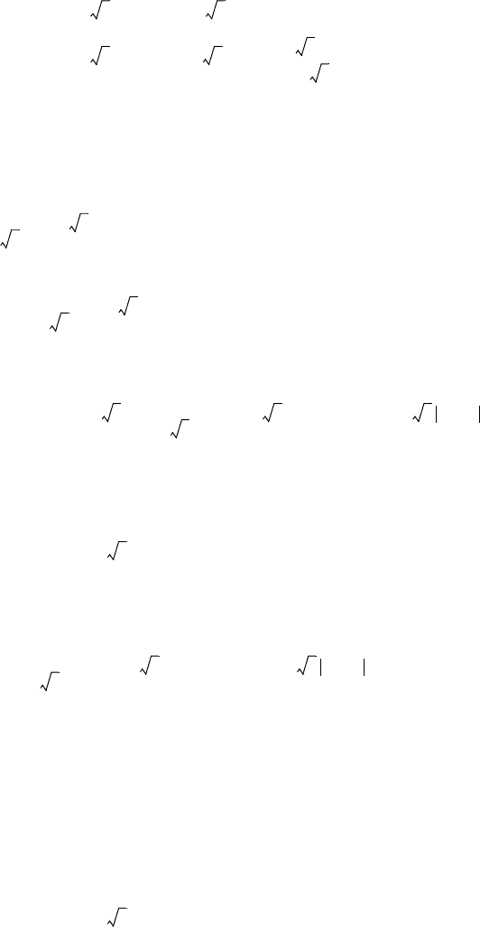
The next problem we shall discus, is the field diffusion in the half-space

(Fig. 6.18). Again, this is given by the solution of the equation

(6.90)

where the boundary conditions are now

(6.91)

, (6.92)

and the initial condition is

(6.93)

As before, for we use (6.79)

(6.94)

with the general solution similar to (6.80),

(6.95)

Only the lower boundary of the integral (6.80) was changed from to

. The reason is that this problem only deals with the positive half-space.

Again, we choose

(6.96)

and in analogy to (6.82) one obtains

ξ 0>

Fig. 6.18

κ 0≠κ 0=

ξ 0>ξ 0< ξ 0=

vacuum conductive medium

∂

ξτ,()

τ∂

∂

ξτ,()=

ξτ,()[]

ξ 0

0 τ,()f τ()==

ξτ,()[]

ξ∞→

∞τ,()finite==

ξτ,()[]

τ 0=

ξ 0,()h ξ()==

ξ p,()

∂

ξ p,()pB

ξ p,()h ξ()–=

ξ p,()A

pξ–[]exp A

+ pξ[]exp h ξ

()

p ξξ

–()sinh

-------------------------------------

∫

–+=

∞–=

h ξ() B

δξ ξ'–()=

370 Time Dependent Problems I (Quasi Stationary Approximation)

(6.97)

From this and the two boundary conditions (6.91) and (6.92), it follows that

(6.98)

and

(6.99)

entirely in accordance with (6.85). Eliminating from (6.98) yields

(6.100)

Finally, with (6.97), (6.99), and (6.100), one obtains the solution to our problem in

the p-domain:

(6.101)

The result needs to be interpreted. We will examine each of the two terms of

individually, since each represents an entirely different cause. If ,

that is, there is no initial field ( ), then

(6.102)

This equation describes the fraction of the field which diffuses from the surface

into the half-space due to the boundary condition at . It shall be explained in

Sect. 6.5.2. Conversely, if while , then

(6.103)

This represents the fraction that stems from the initial condition and which satisfies

the boundary condition at the surface . It will be discussed in

Sect. 6.5.3.

6.5.2 Field Diffusion from the Surface into a Half-space (Impact of

the Boundary Conditions)

If we remove the fraction of the field that is introduced by the initial condition,

what remains is

(6.104)

ξ p,()

-------------------

pξ–[]exp C

pξ[]exp+ for 0 ξξ'<≤

pξ–[]exp C

pξ[]exp

p ξξ'–()[]sinh

-----------------------------------------–+ for 0 ξ' ξ .<≤











+()f

p()=

2 p

----------

pξ'–[]exp=

p()

----------

2 p

----------

pξ'–[]exp–=

ξ p,()f

p() pξ–[]exp

2 p

----------

p ξξ'+()–[]exp– p ξξ'––[]exp+{}.+=

ξ p,() B

h ξ() 0=

ξ p,()f

p() pξ–[]exp=

ξ 0=

p() 0= B

0≠

ξ p,()

2 p

----------

p–()ξξ'+()[]exp– p ξξ'––[]exp+{}=

0 p,()0= ξ 0=

ξ p,()f

p() pξ–[]exp=

6.5 Diffusion of a Field in a Half-Space 371

Let us start with the special case of a δ-function

(6.105)

Then

(6.106)

and

(6.107)

This can be transformed back into the time domain (see table 6.1)

(6.108)

This is the solution to the problem of a very strong field, acting very briefly at the

surface at the time . Now, we consider the general boundary condition ,

which can be assumed as the superposition of many δ-functions:

(6.109)

Each one expands according to the result in (6.108), with the final result

(6.110)

(6.111)

With this, we have reduced the problem of a completely general boundary

condition to an integral transform, which maps the field at the surface onto the field

inside. It achieves this by means of Green’s function given in eq. (6.108).

Notice that we have initially chosen a δ-function as the boundary condition

and then obtained the solution (6.110) by superposing many δ-functions. One could

have chosen a more formal approach, deriving (6.110) directly from (6.104) by

means of the convolution theorem (6.53), (6.54). This is justified because of (see

Tab. 6.1)

(6.112)

f τ() B

δτ τ'–()=

p() B

δτ τ'–() pτ–()exp τd

∞

∫

pτ'–()exp==

ξ p,()B

pτ'– pξ–[]exp=

ξτ,()

0 for ττ'<

4 ττ'–()

--------------------

–exp

2 πτ τ'–()

--------------------------------------------------

for 0 τ' τ .<≤











τ' f τ()

f τ() f τ

()δττ

–()τd

∞

∫

ξτ,() f τ

()

4 ττ

–()

----------------------

–exp

2 πττ

–()

---------------------------------------------

∫

xt,() ft

()

x µκ

µκ

4 tt

–()

--------------------

–exp

2 π tt

–()

-------------------------------------------------------

∫

1–

pξ–()exp{}

4τ

-----

–exp

2 πτ

-----------------------------=

372 Time Dependent Problems I (Quasi Stationary Approximation)

Before, we performed the superposition task in an intuitive way. Now, the

convolution theorem does the job of supperpositioning the individual δ-impulses,

which makes up the function . Eq. (6.110) describes the field’s spatial and

temporal progress in the half-space for an arbitrary field given at the surface, if the

half-space is initially field free. Let us consider the simple example of a field that

increases step-like, at time and then remains constant:

(6.113)

The field is then

(6.114)

Introducing the new variable u

(6.115)

makes

(6.116)

and substituting gives

and with natural dimensions

(6.117)

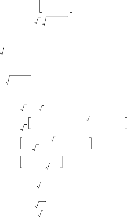
Here, we have introduced the so-called error function (erf) (Fig. 6.19) and its

complementary function the error function complement (erfc):

f τ()

τ 0=

f τ()

0 for τ 0<

for 0 τ .≤







ξτ,()B

4 ττ

–()

----------------------

–exp

2 πττ

–()

---------------------------------------------

∫

2 ττ

–()

--------------------------=

--------

4 ττ

–()

-----------------------------=

ξτ,()B

-------

–[]exp ud

ξ 2 τ⁄

∞

∫

-------

–[]exp ud

∞

∫

–[]exp ud

ξ 2 τ⁄

∫

–=

ξτ,()B

-------

–[]exp ud

ξ 2 τ⁄

∫

–=

1erf

2 τ()

---------------





–=

erfc

2 τ

----------





xt,() B

erfc

x µκ

2 t

--------------





6.5 Diffusion of a Field in a Half-Space 373

(6.118)

. (6.119)

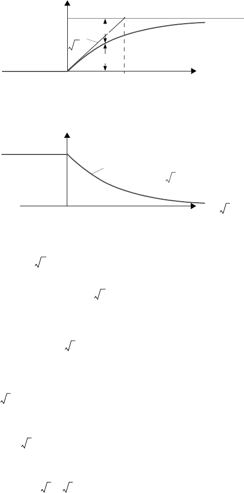
These describe how the field, applied to the surface at time and held

constant thereafter, penetrates the half-space (Fig. 6.20). It is remarkable and an

example for the above mentioned similarity theorems (Sect. 6.2.3), that the field

only depends on and not on the parameters and individually. The

field maintains its principal shape at all times (Fig. 6.20), Stretching more and

more as time increases. When

the value for erfc is

In a rough estimate, it can be stated that within the time , the field has only

reached as far as to the location

(6.120)

Fig. 6.19

erfc x()

erf x()

-------

erf x()

-------

–[]exp ud

∫

erfc x() 1erfx()–

-------

–[]exp ud

∞

∫

t 0=

Fig. 6.20

2 τ

----------

erfc

2 τ

----------





ξ 2 τ()⁄ ξτ

2 τ

----------

0.48≈

erfc

2 τ

----------





---=

τ B

ξ 20.48τ⋅τ≈≈