Lehner G. Electromagnetic Field Theory for Engineers and Physicists

Подождите немного. Документ загружается.

374 Time Dependent Problems I (Quasi Stationary Approximation)

its half width. When returning to the variables with natural dimensions x and t, then

with (6.66) we find how far the field (more precisely half of the field) has

penetrated the half-space

(6.121)

and the time it takes to do so is

(6.122)

This complies with our previous estimates (6.39) and (6.43). This simple example

shall be sufficient for us here, but we will return in a later section (Sect. 6.5.4) to

discuss the problem of the skin effect for the case of a field or current, periodic in

time.

6.5.3 Diffusion of the Initial Field in the Half-Space (Impact of Initial

Values)

The field according to (6.103) is

(6.123)

We examine the second term first. We know it very well from Sect. 6.4, eq. (6.86).

The related time function according to (6.88) is

(6.124)

The first term in (6.123) is of the same kind, at least concerning its effect in the

region , . It describes a field in the positive half-space, which one can

picture as a δ-function-like initial field at location :

(6.125)

The two fields mutually cancel at , which satisfies the boundary condition

there. This is an example of an “image” field, which is necessary to satisfy the

boundary conditions. Nevertheless, this image field is of a different kind than

previous images. In the positive half-space at the time , one has the field

(6.126)

and in the negative half-space ( ), we have the field

(6.127)

which is, of course, of fictitious nature.

µκ

-------≈

t µκx

≈

ξ p,()

– p ξξ'+()–[]exp

2 p

-----------------------------------------------------

p ξξ'––[]exp

2 p

-----------------------------------------------+=

ξτ,()B

ξξ'–()

4τ

--------------------

–exp

4πτ

----------------------------------------

ξ 0>ξ'0>

ξξ'–=

ξτ,() B

ξξ'+()

4τ

--------------------

–exp

4πτ

-----------------------------------------

–=

ξ 0=

τ 0=

ξ 0,()B

δξ ξ'–()=

ξξ'–=

ξ 0,() B

δξ ξ'+()–=

6.5 Diffusion of a Field in a Half-Space 375

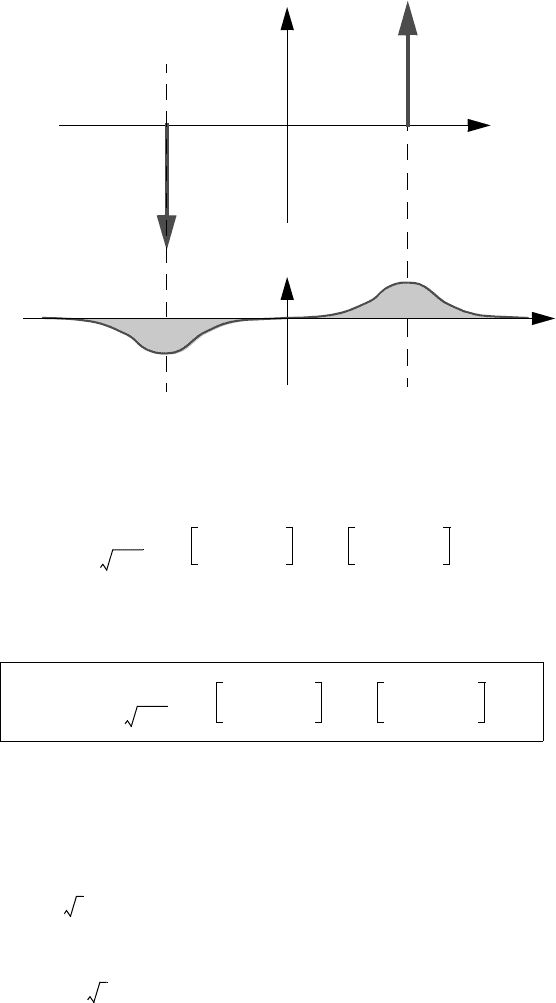
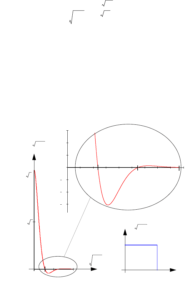
Both fields widen with increasing time to Gaussian curves ((Fig. 6.21). The

overall field at the time τ in the positive half-space is

(6.128)

In the negative half-space, this field is only fictitious. The real field there is

actually zero . If there is an arbitrary initial field , then we need to add

all fractions (in analogy to the discussion of Sect. 6.4).

(6.129)

This represents the general solution of the current problem.

Consider a simple, special case as an example:

(6.130)

Substituting

(6.131)

and

(6.132)

gives

Fig. 6.21

ξ 0,()

ξτ,()

4πτ

-------------

ξξ'–()

4τ

--------------------

–exp

ξξ'+()

4τ

--------------------

–exp–







0= h ξ()

ξτ,()

h ξ

()

4πτ

-------------

ξξ

–()

4τ

----------------------

–exp

ξξ

+()

4τ

----------------------

–exp–







∞

∫

h ξ() B

ξξ

2 τ

--------------=

--------

2 τ

----------

±=

376 Time Dependent Problems I (Quasi Stationary Approximation)

i.e.,

(6.133)

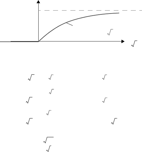
This must be so. It should be easy to see that the resulting field here has to

complement the previously calculated field (6.117) in such a way, that the sum

gives . If there is an initial field inside and a field is applied on the

surface also, then there is the same field everywhere and nothing will happen. If

there is no field applied on the boundary, then eq. (6.133) describes how the field in

the half-space decays. The progression always happens in a similar manner

(Fig. 6.22).

6.5.4 Periodic Field and Skin Effect

Returning to the subject of Sect. 6.5.2, we apply a field, periodic in time to the

surface of the half-space. Complex notation is particularly useful here to simplify

periodic processes. We write

(6.134)

The real part represents the physical field at the surface. Then

(6.135)

and with (6.104)

ξτ,()

-------– u

–[]exp ud

ξ 2 τ⁄

∞–

∫

–[]exp ud

ξ 2 τ⁄

+∞

∫







-------

–[]exp ud

∞–

ξ 2 τ⁄

∫

–[]exp ud

ξ 2 τ⁄

+∞

∫

–







---------

–[]exp ud

ξ 2 τ⁄

∫

erf

2 τ

----------





xt,() B

erf

x µκ

2 t

--------------





Fig. 6.22

erf

2 τ

----------





2 τ

----------

0 τ,()f τ() B

Ωτ()cos i Ωτ()sin+[]B

iΩτ()exp== =

Ωτ()cos

p()

piΩ–

---------------=

6.5 Diffusion of a Field in a Half-Space 377

(6.136)

is the dimensionless angular frequency, where

(6.137)

The before mentioned table of Laplace transforms [5] contains the transform of

(6.136) into the time domain.

(6.138)

For very large times ( )

and therefore the real physical field in the half-space is

(6.139)

The field given by (6.139) remains, after the effects from the initial conditions have

subsided (here, this is the field that vanishes at the beginning). The remaining field

represents the so-called steady state. It alone would not satisfy the initial conditions

at . A different initial condition would cause additional terms which would

decay over time. The steady state will always be the one given by (6.139). The

steady state shall occupy us for now. It shares the periodicity with the applied field,

however, there is a spatial dependent phase shift and the amplitude decreases

(damping) towards the inside of the half-space. Intuitively, both are to be expected.

If the interest is only in the steady state, it can be calculated rather easily. The

starting point is

(6.140)

and the solution has to consist of exponential functions, therefore we try the Ansatz

ξ p,()

piΩ–

---------------

pξ–[]exp=

Ω

Ωτ ωt Ω

µκl

-----------

Ωωµκl

ξτ,()

------

iΩτ() 1 i+()

Ωξ

----------–exp erfc

2 τ

----------1i+()

Ωτ

-------–







exp=

+ 1 i+()

Ωξ

----------exp erfc

2 τ

----------1i+()

Ωτ

-------+







τ∞→

erfc

2 τ

----------1i+()

Ωτ

-------–2=

erfc

2 τ

----------1i+()

Ωτ

-------+0=

ξτ,()B

i Ωτ

Ωξ

----------–





exp

Ωξ

----------–exp=

ξτ,()B

Ωτ

Ωξ

----------–





cos

Ωξ

----------– exp=

τ 0=

∂

ξτ,()

τ∂

∂

ξτ,()=

378 Time Dependent Problems I (Quasi Stationary Approximation)

(6.141)

This requires

(6.142)

Thus, there are two solutions:

(6.143)

Only the sign on the top provides solutions which make physical sense. The bottom

sign would cause a field which diverge for . Although this is a

mathematically correct solution, one excludes it because Physics does not allow for

such a field. Therefore, the field is given by:

(6.144)

Both, the real part as well as the imaginary part can be regarded as solutions. The

real part just represents the previous solution of eq. (6.139). Returning to variables

with dimensions, the field becomes

(6.145)

The phase is constant when

that is, for

(6.146)

This is the phase velocity, which represents the velocity with which the wave

starting at the surface penetrates the half-space. The penetration depth, i.e., the

distance at which the amplitude has fallen to is given by

(6.147)

ξτ,()B

i Ωτ kξ–()[]exp=

– iΩ=

k Ω i– Ω

1 i–

----------





±==

ξτ,()B

i Ωτ

Ω

----

−





Ω

----

−

exp=

ξ∞→

ξτ,()B

i Ωτ

Ω

----

–





Ω

----

–exp=

xt,() B

µκω

----------- x–exp ωt

µκω

----------- x–cos=

ωt

µκω

----------- x–const.=

ωdt

µκω

----------- dx–0=

------

2ω

µκ

-------=

1 e⁄

µκω

----------- d 1=

µκω

-----------=

6.5 Diffusion of a Field in a Half-Space 379

With the exception of the factor , this is in entire harmony with our previous

approximation (6.44). However, because of the very rough approximation in

Sect. 6.2, which did not take into account the geometry of the set-up, we could not

have expected an exact result.

From

follows for the corresponding current

(6.148)

where the trigonometric identity

was used. The time average of the squared current density is

(6.149)

This allows one to determine the average power that is transformed per unit of the

surface of the half-space.

(6.150)

According to (6.148) one writes

(6.151)

and therefore, one gets for the overall current per unit length on the surface

(6.152)

Squaring this and then taking the time average gives

(6.153)

Imagine that this current flows according to eq. (6.147) within the depth d, then the

related power per unit area is

H∇× g=

xt,()

t∂

∂

xt,()–=

µκω

----------- x– ωt

µκω

----------- x–

---+cosexp=

αcos αsin–2α

---+





cos=

x()

µκω

-------------------

2µκωx–[]exp=

x()

---------------

∞

∫

µω

-------

2µκωx–[]exp xd

∞

∫

µω

22µκω

----------------------

µω

22κ

--------------

x()xd

∫

x∂

∂H

∫

– H

a() H

b()–==

x()xd

∞

∫

0() H

∞()– H

ωtcos==

x()xd

∞

∫





-------=

380 Time Dependent Problems I (Quasi Stationary Approximation)

(6.154)

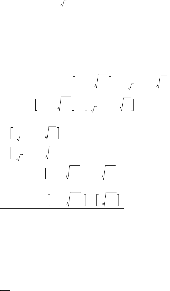
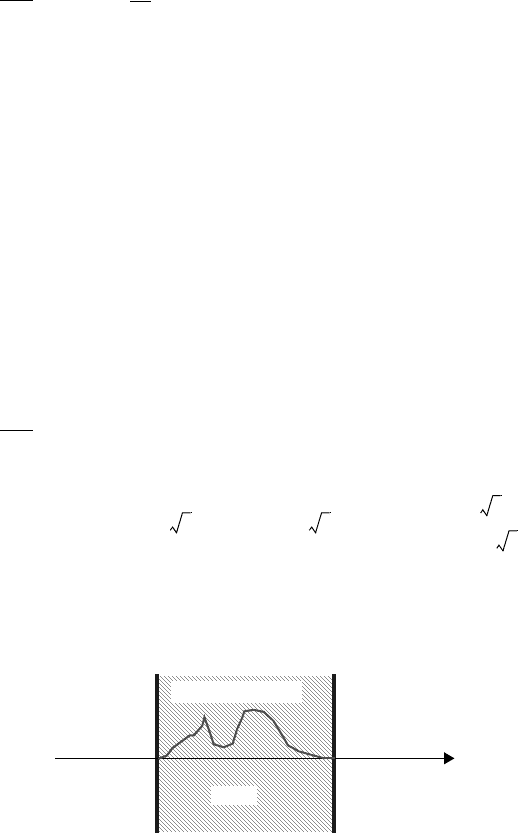
This just describes the power calculated in eq. (6.150), which conjures up a

scenario where the entire, effective current, flows with a uniform current density in

a layer at the surface of thickness d. Fig. 6.23 compares for example for the time

the actual current distribution (Fig. 6.23a) with that of our model

distribution (Fig. 6.23b).

0.0306

0.34

0.71

0.707

0.031

gx()

8.638

0 x

0.04

0.03

0.02

0.01

0.02

0.03

fx1()

zt()

PNZ

----------- x

-- -

------

11S

---------

------ -

----------

b)a)

x 0

PNZ

---------------------- -

x 0

PNZ

---------------------- -

------

Fig. 6.23

-------

R⋅

-------

κd

------

⋅

2κ

µκω

-----------

-----------------------

µω

22κ

-------------------== =

t 0=

6.6 Field Diffusion in a Plane Plate 381

6.6 Field Diffusion in a Plane Plate

6.6.1 General Solution

Now, we discuss the problem of a plane plate of thickness d, as illustrated in

(Fig. 6.24). Then one has to solve the diffusion equation

(6.155)

with the boundary conditions

(6.156)

(6.157)

and the initial condition

(6.158)

Here, one replaces the arbitrary length l by the thickness of the plate d, i.e.,

(6.159)

and

(6.160)

For , the formula (6.94) applies again

(6.161)

Its general solution by eq. (6.95) is

(6.162)

Fig. 6.24

1 τ,()f

τ()=

0 τ,()f

τ()=

x 0= xd=

xo,()hx()=

κ,

vacuum vacuummedium

∂

ξτ,()

τ∂

∂

ξτ,()=

0 τ,()f

τ()=

1 τ,()f

τ()=

ξ 0,()h ξ()=

µκd

-------------=

---= for 0 ξ 1≤≤

ξ p,()

∂

ξ p,()pB

ξ p,()h ξ()–=

ξ p,()A

pξ–[]exp A

+ pξ[]exp h ξ

()

p ξξ

–()[]sinh

------------------------------------------

∫

–+=

382 Time Dependent Problems I (Quasi Stationary Approximation)

In the p-domain, it has to satisfy the boundary conditions given in (6.156) and

(6.157).

(6.163)

. (6.164)

This determines the constants and , and the final result in the p-domain is

(6.165)

The field has three parts which we will discuss separately. The three parts are due

to the two boundary conditions and the initial condition. It is possible to verify the

correctness of this solution by substituting it into (6.161). That the boundary

conditions (6.163) and (6.164) are satisfied can also be verified by inspection.

6.6.2 Diffusion of the Initial Field (Impact of Initial Condition)

We start our discussion with the last part, i.e., the two terms of (6.165) which stem

from . As we have found before, it is sufficient to study the special case

(6.166)

The reason is that the general case can be reduced to this special case. Without the

terms with and , the field becomes

(6.167)

where we have used the relation

Transforming eq. (6.167) back into the time domain yields

(6.168)

0 p,()f

p()=

1 p,()f

p()=

ξ p,()f

p()

p 1 ξ–()[]sinh

p[]sinh

----------------------------------------

p()

pξ[]sinh

p[]sinh

--------------------------

pξ[]sinh

p[]sinh

--------------------------

h ξ

()

p 1 ξ

–()[]sinh

------------------------------------------

∫

h ξ

()

p ξξ

–()[]sinh

------------------------------------------

∫

–











h ξ()

h ξ() B

δξ ξ'–()=

p() f

p()

ξ p,()

pξ[]sinh p 1 ξ'–()[]sinh

pp[]sinh

-------------------------------------------------------------------

for ξ' ξ >

pξ'[]sinh p 1 ξ–()[]sinh

pp[]sinh

-------------------------------------------------------------------

for ξ' ξ .<











pξ[]sinh p 1 ξ'–()[]sinh p[]sinh p ξξ'–()[]sinh–

pξ'[]sinh p 1 ξ–()[]sinh=

ξτ,() 2B

nπξ()sin nπξ'()sin n

τ–[]exp

n 1=

∞

∑

6.6 Field Diffusion in a Plane Plate 383

Its proof shall be postponed until the end of this section. Now, one can write the

general solution for an arbitrary initial field

(6.169)

This result is in the form of a Fourier series. One could have derived this without

the Laplace transform, had we chosen to start with an Ansatz of the form of a

Fourier series. One can verify by inspection that eq. (6.169) solves our problem.

First, every term satisfies the partial differential equation (6.155) and the boundary

conditions for and . Furthermore, for the time ,

the field is

(6.170)

that is, it satisfies the initial condition.

As specific example, consider

(6.171)

for which one first finds

(6.172)

and therefore

(6.173)

The result is in the form of an infinite series and converges extremely well if the

time is not too small. For a sufficiently large times, the first term of the series

already represents a rather useful approximation. For

(6.174)

(6.175)

one has

(6.176)

that is, the field behaves as indicated in Fig. 6.25. Conversely, for small times, the

series does not converge well. On a side note, it shall be mentioned that this series

is closely related to the so-called θ-functions. There are relations between

ξτ,() 2 nπξ()sin h ξ

() nπξ

sin ξ

∫







τ–[] exp

n 1=

∞

∑

ξτ,()0= ξ 0= ξ 1= τ 0=

ξ 0,() h ξ

()

∫

2 nπξ

sin nπξ()sin

n 1=

∞

∑

dhξ

()

∫

δξ ξ

–()ξ

d==

h ξ()=

h ξ() B

nπξ

sin

∫

nπ

------

11–()

–[]=

ξτ,()

nπ

---------

11–()

–[]nπξ() n

τ–[]expsin

n 1=

∞

∑

µκd

-------------

------»=

µκd

-------------»

xt,()

---------

πx

------





µκd

-------------–expsin≈