Lehner G. Electromagnetic Field Theory for Engineers and Physicists

Подождите немного. Документ загружается.

424 Time Dependent Problems II (Electromagnetic Waves)

. (7.85)

Both statements may be formally expressed by

(7.86)

From it follows immediately

and

Furthermore

(7.87)

With this, the two statements (7.81) and (7.82), together with the wave equations

(7.79) and (7.80), again yield the dispersion relation (7.83). Next we will apply

Maxwell’s equations to the statements (7.81) and (7.82). Starting with (7.4), letting

gives

(7.88)

Consequently, and have to be perpendicular to each other, i.e., the wave has

to be transverse relative to . It also has to be transverse relative to , since it

follows from (7.3) that

(7.89)

Furthermore, from (7.2) it follows that

and thus

(7.90)

As a special case, this formula contains relation (7.31), which was previously

derived in a much more tedious manner. The generalization is grounded in the fact

that according to (7.83), k is generally not a real valued vector. Finally, one needs

to consider (7.1), which, when used in conjunction with (7.6) yields

(7.91)

Eq. (7.90) allows to eliminate B and obtain

Finally, with (7.88) one finds

E∇×

x∂

∂

y∂

∂

z∂

∂

– ik

–

ikE×–== =

∇ ik –=

divEE∇• ikE•–==

curlEE∇× ikE×–==

∆∇∇•∇

ik–() ik–()• k

–=== =

ρ 0=

D∇• ε E∇• iεkE•–0== =

B∇• ikB•–0==

E∇× ikE×–

t∂

∂B

– iωB–===

kE×

-------------=

ik– B×µκE µεiωE+=

kE×

-------------





×–

----– kk E•()Ek k•()–[]µκE µεiωE+==

7.2 Plane Waves in a Conductive Medium 425

(7.92)

i.e., again the dispersion relation (7.83).

With this, we have now again derived the properties for the special case of a

plane wave in an insulator ( ), however, this time in a formally much shorter

and more elegant way than above. The current approach for the derivation

highlights specifically the transverse nature of the wave with respect to E and is a

consequence of E being source free. Remember that we had assumed that .

The fact that E and B are perpendicular to each other as expressed in (7.90), is an

immediate consequence of the law of induction.

For the case , the dispersion relation (7.83) reduces to a result we

already know:

The relation is more complicated for a conductor. There are a number of different

cases, of which we shall restrict our discussion to only two limiting cases.

7.2.2 The Process is Harmonic in Space

If a process is harmonic in space, then k is real valued and as a consequence, is

complex valued. If we identify the real part of with and its imaginary part

with , then

(7.93)

Rewriting eq. (7.83) using this new assignment gives

For this to be true, both, the real and the imaginary part have to vanish

independently

(7.94)

(7.95)

Solving (7.95) for gives

(7.96)

Inserting this in (7.94) and solving for gives

(7.97)

Definition (7.93) requires that is real. This is only true if

-------

E µκE µεiωE+=

κ 0=

ρ 0=

κ 0=

µκω

------==

ω ck=

ωη

ωηiσ

µε η

2ησ

i σ

–+()µκiησ

–()– k

–0=

– κµσ

εµη

εµσ

–++ 0=

ηκµ–2εηµσ

+0 .=

ηκµ

2εηµ

-------------

2ε

-----==

εµσ

κµσ

–+

εµ

--------------------------------------------±

εµ

------

4ε

--------–±==

426 Time Dependent Problems II (Electromagnetic Waves)

(7.98)

Then, the wave becomes

(7.99)

This means that for the wave, plays the role of the real valued angular frequency

while introduces exponential decay over time (damping).

Conversely, if

(7.100)

then, becomes purely imaginary and we may write

(7.101)

Substituting this into (7.83) gives

(7.102)

The two solutions when solving the quadratic equation (7.102) for are

(7.103)

Finally, the wave becomes

(7.104)

To compare the two waves of (7.99) and (7.104) with each other is revealing.

While the wave propagates for sufficiently large wave numbers (condition (7.98)),

this is not the case for small wave numbers (condition (7.100)). The root cause for

this peculiar behavior is that the diffusion process and the wave propagation

process compete with each other. Take the wave equation in its form (7.79) or

(7.80), then we find that in the statement of the form (7.81) and (7.82), the

diffusion term basically behaves like

while the wave propagation term behaves like

If, for example, κ is very small, ε very large, then the diffusion term can be

neglected. Then, according to (7.98), the wave propagates with the phase velocity

for almost all wave numbers k (except for extremely small ones). Conversely,

if κ is very large and ε very small, then the diffusion term dominates. Now, for

almost all wave numbers k (except for extremely large ones), the resulting

expression has now the form of (7.104), which describes an exponentially decaying

field and not a propagating wave.

4ε

---------

≥

i η iσ

+()tikr•–[]exp=

i ηt kr•–()[]exp σ

t–[]exp=

4ε

---------

ω iσ

– κµσ

εµσ

–+0=

2ε

-----

4ε

--------

εµ

------–±=

i– kr•()[]exp σ

t–[]exp=

µκω

µεω

η k⁄

7.2 Plane Waves in a Conductive Medium 427

7.2.3 The Process is Harmonic in Time

For a harmonic process, which in practise is the more important case, ω is real,

while k is complex. One may write

(7.105)

and with eq. (7.83) obtains

Separating the real and imaginary part gives

(7.106)

. (7.107)

Solving for α gives

and the quadratic equation in is

(7.108)

Solving for β yields four solutions:

In the definition, we have required that β is real. Consequently for the term under

the radical, only the positive sign can be considered. Therefore

(7.109)

With this and eqs. (7.106), (7.107) one obtains for α:

(7.110)

It shall be noted, that one could allow for imaginary values for β. However, this

makes α imaginary as well and comparison of the results reveals that this does not

provide anything new. Merely, α and β exchange their roles.

Using eqs. (7.105), (7.109), (7.110) in (7.81) gives

(7.111)

having assumed that k is a vector in z-direction. This makes the real part of k,

namely β, responsible for propagation of the wave, while its imaginary part α,

controls the damping. Therefore α is called damping constant, and β the phase

constant. Eq. (7.111) describes a damped plane wave. The plane

represents both: planes of constant phase, as well as planes of constant amplitude.

A wave with these properties is also called a homogeneous wave.

k β iα–=

εµω

κµωi– β

2αβi– α

–()–0=

– α

εµω

++ 0=

2αβ κµω–0=

κµω

2β

-----------=

εµω

–

-------------------–0=

βω

εµ

------

------------+ ±





±=

βω

εµ

------

------------+1+





±=

αω

εµ

------

------------+1–





±=

i ωt βz–()[]exp αz–[]exp=

z const.=

428 Time Dependent Problems II (Electromagnetic Waves)

This is by no means the most general case. This is obtained if

(7.112)

where and are vectors for which the dispersion relation has to hold, i.e.,

(7.113)

If the two vectors and are parallel, then the appropriate choice of coordinate

system allows to arrive at the same expression as stated in (7.111), and thus one

obtains a homogeneous wave in the just defined sense. The planes of constant

phase are perpendicular to . The planes of constant amplitude are perpendicular

to . If the two vectors point in different directions, then the result is an

inhomogeneous wave. In order to be able to provide a simple example, let

in (7.113). This forces and to be perpendicular. One may assume, for

example, that

(7.114)

which results in the wave

(7.115)

For the relation between b and a we have

(7.116)

Inhomogeneous waves are not transverse, as (7.90) clearly shows. Moreover, they

are not plane waves in the sense of our definition because the amplitude is not

constant in the planes where the phase is constant. Nevertheless, inhomogeneous

waves are important. Oftentimes, they are necessary to satisfy boundary

conditions, e.g., for reflection problems. We will come back to such cases.

The magnetic field that belongs to the wave described by (7.111) results from

(7.90). B is perpendicular to E. However, there is a phase difference between B and

E because k is a complex vector. There was no phase difference in the ideal

insulator ( ). If the electric field is

then the magnetic field becomes

Notice that B has only a y-component

If is real valued, then the electric field expressed in real value notation is

(7.117)

and the magnetic field is

k b ia–=

µεω

µκiω– b

i2ab• a

––()–0=

κ 0=

k b 0 ia–,,〈〉=

i ωtbx–()[]exp az–[]exp=

– a

µεω

++ 0=

κ 0=

00,,〈〉=

00β iα–,,〈〉

--------------------------------

00,,〈〉i ωt βz–()[]exp αz–[]exp×=

0β iα–()E

0,,〈〉

i ωt βz–()[]exp αz–[]exp

----------------------------------------------------------------

β iα–()E

-----------------------------

i ωt βz–()[]exp αz–[]exp=

ωt βz–()cos αz–[]exp=

7.2 Plane Waves in a Conductive Medium 429

i.e.,

Let

and thus

(7.118)

which yields

(7.119)

where

(7.120)

and

(7.121)

Letting results in the previously discussed case of the ideal insulator.

We will discuss two limits: If

or expressed differently by using the relaxation time from Sect. 4.2, eq. (4.23)

then the dominant term in the wave equation is

the diffusion term. the wave propagation term.

ℜe

--------

β iα–()ωt βz–()cos i ωt βz–()sin+[]αz–[]exp







--------

βωt βz–()cos αωt βz–()sin+[]αz–()exp=

--------

-----------------------

ωt βz–()cos=

-----------------------

ωt βz–()sin αz–() .exp+

----------------------- ϕsin=

----------------------- ϕcos=

ϕtan

---=

ωt βz– ϕ–()cos αz–[]exp=

--------

+ E

µε 1

------------+

--------

------------+

κ 0=

ωε κ« κωε«

ωt

1,«1ωt

430 Time Dependent Problems II (Electromagnetic Waves)

Using (7.109) and (7.110) yields

and for the phase velocity

The dominating property in this case is

The material is therefore called a

Whether a particular material should be considered more in terms of a conductor or

an insulator with respect to a particular wave, does not only depend on the material

constants and , but also on the frequency of the wave under consideration. The

become apparent for frequencies sufficiently

Apprehensibly, the reason lies in volume charge carrier mobility. When the

frequency of the oscillating electric field is

the motion of the charges is

to be able to cancel the field created by the displaced volume charges.

It is impossible for an electrostatic field to exist in a conductor (Sect. 2.6),

while slowly oscillating fields can penetrate the conductor only a very small

distance. Even within the distance of one wave length, they are damped by a factor

of , which is the result of (7.111) for . Otherwise, the

results we obtain here for the limit of small frequencies are identical to those

obtained in Sect. 6.5.4. Take note of eq. (6.145).

The energy lost by damping is transformed into heat. The proof can be

performed using the energy principle, which we will forgo here.

characteristics of a conductor . characteristics of an insulator.

conductor. not an ideal insulator.

conductor properties insulator properties

small. large.

small, large,

sufficiently fast not fast enough

αβ

µκω

-----------±≈≈

---

---±≈

βωµε1

8ω

---------------+





±≈

----

2ω

µκ

-------±≈=

1±

µε 1

8ω

---------------+





-----------------------------------------

≈

8ω

---------------–





µε

----------------------------------

.≈

κε

2π–()exp 2 10

3–

⋅≈αβ=

7.3 Reflection and Refraction 431

7.3 Reflection and Refraction

7.3.1 Reflection and Refraction for Insulators

Let a plane wave be incident on a plane boundary between two insulators (“media

boundary”), then the various boundary conditions for E, D, H, B have to be

satisfied.

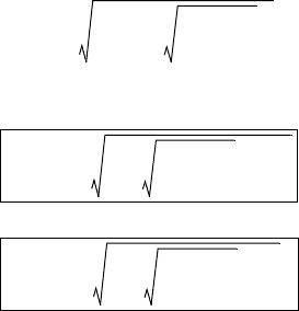
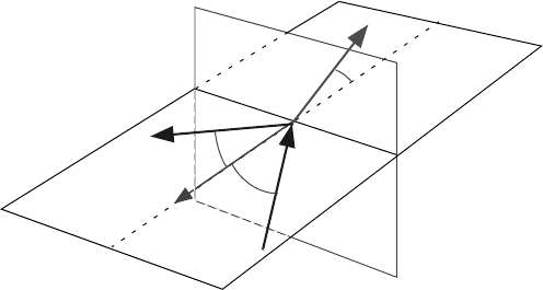
Fig. 7.9 illustrates this. The boundary conditions can be satisfied, if one

assumes that besides the incident wave ( ), there is also a wave reflected back

into medium 1 ( ), and a transmitted wave ( ) into medium 2. Disregarding the

case of total internal reflection, which we will discuss later, one has a wave of the

form:

(7.122)

(7.123)

. (7.124)

Certain field components have to be continuous at the media boundary. This results

in certain relations between , and . Because the boundary conditions

have to be satisfied at all times and for every point on the boundary, all the

phases of the exponential functions in (7.122) through (7.124) have be equal. In

particular, it must be

(7.125)

Consequently, there is only one frequency in both media. Without limiting the

generality, it may be assumed that the origin of the coordinate system lies in the

boundary between the media. Then the vectors for all points on the boundary

lay entirely on the boundary itself. Therefore, it has to be

(7.126)

Fig. 7.9

media boundary

κ 0=

i ω

t k

r•–()[]exp=

i ω

t k

r•–()[]exp=

i ω

t k

r•–()[]exp=

, E

ω===

• k

•==

432 Time Dependent Problems II (Electromagnetic Waves)

From this we first obtain

(7.127)

Consequently, the vector is perpendicular to the boundary and we may

write

(7.128)

where A is a constant. Therefore, the three vectors lie in a plane, the so-

called plane of incidence, they are coplanar. Also, the two vectors and have

the same magnitude, i.e., they share the same frequency and the

same medium (medium 1). The components of and which are parallel to the

boundary are obviously the same. Therefore, both angles are the same

(7.129)

This is the well-known law of refraction. Furthermore

(7.130)

Therefore, besides the three vectors , also lays in the plane of

incidence. However, and have a different magnitude. From the dispersion

relation (7.39) one finds that

(7.131)

. (7.132)

It follows from (7.130) that the tangential components of and must be equal,

i.e.,

and applying (7.131) and (7.132) gives

Renaming

(7.133)

and

(7.134)

yields Snell’s law:

(7.135)

–()r

• 0=

–

– An=

n,,

ωω

–()r

• 0=

n,, k

----

---------------=

----

---------------=

sin k

sin=

----

sin

-------------

ωε

--------------------

---------------== =

-----

εµ

--------------- ε

== =

sin

--------------

-----

7.3 Reflection and Refraction 433

7.3.2 Fresnel’s Equations for Insulators

Now we need to derive the relations between the amplitudes of the waves (7.122)

through (7.124) from the boundary conditions for the fields. To do so, we need to

distinguish two cases, whether the vector of the incident electric field lies in the

plane of incidence, i.e., is parallel to it, or whether it is perpendicular to the plane of

incidence. Every wave can be decomposed into these two components. We call one

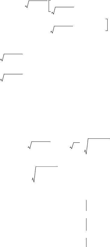
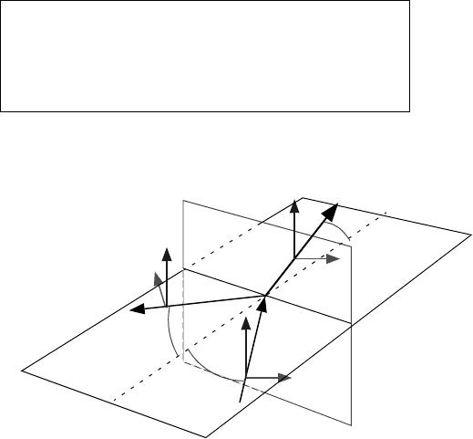
case parallel polarization and the other perpendicular polarization. The discussion

shall start with perpendicular polarization (Fig. 7.10). The components of E and H

parallel to the boundary have to be continuous at the boundary. It must be

(7.136)

. (7.137)

With (7.32), (7.33) we get

(7.138)

and using this with (7.137) gives

(7.139)

With (7.136) and (7.139), we have two equations for two unknowns and

( is considered as given). Solving for these yields

(7.140)

Fig. 7.10

κ 0=

+ E

cos H

cos– H

cos=

Z⁄=

–()

cos

---------------

cos

---------------

--------





⊥

cos

---------------

cos

---------------–

cos

---------------

cos

---------------+

-------------------------------------

cos Z

cos–

cos Z

cos+

-------------------------------------------------