Lehner G. Electromagnetic Field Theory for Engineers and Physicists

Подождите немного. Документ загружается.

494 Time Dependent Problems II (Electromagnetic Waves)

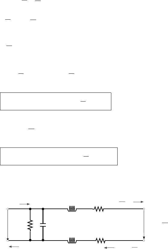
of Fig. 7.38 is a special case thereof. The two-gate shown in Fig. 7.39 corresponds

to a line element of length dz.

The quantities are in the same order: conductance, capacitance,

inductance, resistance, all per unit length of the transmission line. With it

follows from Fig. 7.39:

(7.429)

. (7.430)

Differentiating the first equation for z yields:

Substituting from the second equation yields

or after rearranging

(7.431)

Similarly for the second equation

and substituting from the first equation yields

(7.432)

Notice that and satisfy the same telegrapher's equation. In the

simplest case, the line is free of losses, this means that

Fig. 7.39

---

L'dz

Vz()

---

R'dz

Iz()

z∂

∂I

dz+

Iz()

---

L'dz

---

R'dz

Iz()

z∂

∂I

dz+

Vz()

z∂

∂V

dz+

G'dz C'dz

G' C' L' R',,,

dz 0→

G'VC'

t∂

∂V

z∂

∂I

++ 0=

t∂

∂I

R'I

z∂

∂V

++ 0=

z∂

∂V

∂

∂t∂z

-----------

∂

∂z

--------++0=

∂V ∂z⁄

G' L'

t∂

∂I

– R'I–





∂

∂t

----

t∂

∂I

– R'I–





∂

∂z

--------++0=

∂

∂z

--------

L'C'

∂

∂t

--------

R'C' L'G'+()

t∂

∂I

G'R'I++ =

∂

∂t

----

∂I

∂z

-----

z∂

∂I

∂

∂z

---------++ 0=

∂I ∂z⁄

∂

∂z

---------

L'C'

∂

∂t

---------

R'C' L'G'+()

t∂

∂V

G'R'V++ =

Izt,() Vzt,()

7.11 The Wave Guide as a Variational Problem 495

(7.433)

(7.434)

and therefore

(7.435)

. (7.436)

One can prove that it must always be

(7.437)

We will skip the general proof. For the case of the coaxial cable, (7.437) can be

verified by means of eqs. (2.98) and (5.210), when replacing by and by

For V we try the following Ansatz

(7.438)

and obtain from (7.435)

i.e., the usual dispersion relation for TEM waves in multiply connected wave

guides (for example, in a coaxial cable, although above relation is by no means

limited to the coaxial cable).

The current I creates the magnetic field (in case of the coaxial cable H is

purely azimuthal), the EMF V creates the electric field between inside and outside

conductor (for the coaxial cable, E is purely radial).

We will not advance any deeper into the matter of transmission theory, as our

purpose was only to highlight the relation between transmission theory and field

theory.

7.11 The Wave Guide as a Variational Problem

From a mathematical perspective, solving wave guide problems means to solve the

Helmholtz equation in its form (7.344) or (7.350)

(7.439)

where is the two-dimensional Laplacian, here in Cartesian coordinates:

(7.440)

We might as well use a different coordinate system. In any case, according to

(7.349), the boundary mandates for TM waves

(7.441)

G'0=

R'0=

∂

∂z

--------- L'C'

∂

∂t

---------

∂

∂z

-------- L'C'

∂

∂t

--------

L'C' εµ=

εµ

Vzt,() V

i ωtk

z–()[]exp=

– εµω

+0=

∆

xy,()NΠ

xy,()+0=

∆

∂

496 Time Dependent Problems II (Electromagnetic Waves)

and according to (7.355) for TE waves

(7.442)

From solving a number of example problems above, we found that there are

only certain functions that satisfy the boundary conditions. Related are certain

values of N. These functions are the eigenfunctions and the related N-values are the

eigenvalues of the problem. The eigenfunctions form a complete system of

orthogonal functions (Sect. 3.6). These are trigonometric functions in case of the

rectangular wave guides and in case of circular cylindrical wave guides, these are

Bessel functions. These functions are the basis to expand other functions in form of

Fourier or Fourier-Bessel series, as we have done multiple times above.

Now address the eigenvalues by

and their related eigenfunctions by

where we still refer to the z-component, but have dropped the index z to simplify.

The order of the eigenvalues shall be such that

(7.443)

It is possible to show that the various eigenfunctions belonging to different

eigenvalues are, indeed, orthogonal to each other. Also possible is to have several

eigenfunctions to the same eigenvalue where the eigenfunctions are still

orthogonal. Then the eigenfunctions and eigenvalues are said to be “degenerate”.

For simplicity reasons, we will exclude this case from our discussion, which does

not limit the possible conclusions we will draw. Now, we will consider two

eigenfunctions and with their eigenvalues and . With (7.439), one

finds:

(7.444)

. (7.445)

Multiplying the first equation by and the second by yields

(7.446)

. (7.447)

Then we subtract them and integrate

(7.448)

where the area of integration is the cross section. Analogous to Green’s theorem in

the three-dimensional space (3.47), there is a Green’s theorem for the plane (which

can be derived from the one in three-dimensional space). It reads as follows (see

Sect. 3.4.2):

n∂

∂Π

…,,,

…<<<<

∆

+0=

∆

+0=

∆

+0=

∆

+0=

∆

–()Ad

∫

–()Π

∫

–=

7.11 The Wave Guide as a Variational Problem 497

(7.449)

Therefore, with the boundary conditions (7.441) or (7.442), we have

i.e., requires that

(7.450)

which proves our claim that the two functions and are orthogonal.

Now, consider an arbitrary, well behaved function and its series

representation:

(7.451)

For the case of a rectangular wave guide, this would be a two-dimensional Fourier

series, for the case of a TM wave in a circular cylinder, this would be a double

series, where the -dependency is represented by a Fourier series while the r-

dependency expands in a Fourier-Bessel series.

Let us investigate the following expression:

(7.452)

Using (7.451) we obtain

(7.453)

We have used the fact that (7.450) permits us to write

∆

–()Ad

∫

n∂

∂Π

n∂

∂Π

–





∫

–()Π

∫

– Π

n∂

∂Π

n∂

∂Π

–





∫

0==

≠

∫

φ a

i 1=

∞

∑

φ∆

φ Ad

∫

----------------------–=

i 1=

∞

∑

∆

k 1=

∞

∑

∫

ik, 1=

∞

∑

∫

-------------------------------------------------------------–=

ik, 1=

∞

∑

∫

ik, 1=

∞

∑

∫

-------------------------------------------------------

ik, 1=

∞

∑

ik, 1=

∞

∑

---------------------------------------------==

i 1=

∞

∑

i 1=

∞

∑

----------------------------

i 1=

∞

∑

i 1=

∞

∑

-----------------------------

≥ N

498 Time Dependent Problems II (Electromagnetic Waves)

(7.454)

where is an arbitrary normalizing factor. We have determined that

(7.455)

The equal sign applies if, and only if

In other words: is nothing else than the lowest value which the expression F

may take and the function for which it assumes this value is the eigenfunction

. Now we have transformed the wave guide problem into a variational problem.

The task is now to find the function that fulfills the given boundary conditions,

while minimizing the expression F. Then, after finding we continue to

determine . Now, we need to find the function which makes the expression F

as small as possible, while still needs to satisfy the given boundary conditions

and, in addition, has to be perpendicular to . This requires and thus

obtain

(7.456)

The equal sign now applies if .

This, from a formal perspective interesting remark, shall conclude the

problem of waves in waveguides. Many more problems in physics, and in

electromagnetic field theory in particular, can be regarded as variational problems.

This is very useful because variation problems are a very good basis for

approximation methods and numerical calculations. We will revisit this subject in

Chapter 8.

7.12 Boundary and Initial Value Problems

In Chapter 6, we discussed the quasi-stationary approximation, while Chapter 7

was dedicated to the complete Maxwellian equations. From a formal perspective,

the quasi-stationary case requires to solve the diffusion equation, in our case the

wave equation, in one form or another. In its general form, the wave equation also

contains a diffusion term. For instance, consider the magnetic field B, then with

(7.9) we write

(7.457)

from which emerges the diffusion equation when neglecting the propagation terms

(7.458)

∫

≥

φΠ

i 2=

∞

∑

i 2=

∞

∑

----------------------------

i 2=

∞

∑

i 2=

∞

∑

-----------------------------

≥ N

φΠ

∇

B µκ

t∂

∂B

– µε

∂

∂t

----------

–0=

∇

B µκ

t∂

∂B

0==

7.12 Boundary and Initial Value Problems 499

At various times, we have discussed the limits of the quasi stationary theory and

the competing effects of diffusion and wave propagation (see Sect. 6.8. and also

Sect. 6.2). We shall revisit this discussion once more. For instance, one can solve

the general wave equation (7.457) by the same methods which we have used in

Chapter 6 to solve the diffusion equation. Then retroactively, we may let ,

which results in an undamped wave propagation in an ideal insulator, or

conversely, let to obtain the limit of diffusion.

To illustrate this, we will revisit two examples which we have already solved

in Chapter 6, but now we include the wave propagation term. First, the problem of

an initial field in the infinite, uniform space (Sect. 6.4) and second, the problem of

the half-space (Sect. 6.5).

At the same time, the solution of these two problems shall demonstrate the

general usefulness of methods previously used to solve initial value and boundary

value problems.

7.12.1 The Initial Value Problem of the Infinite, Uniform Space

The task is to solve the problem given in Sect. 6.4 starting from the wave equation

(7.457). Now, the order of the differential equation with respect to the time is two

and, compared to before, this requires an additional initial value condition. We

want to find for which the wave equation has the form

(7.459)

Furthermore, the initial value and the boundary conditions shall be:

(7.460)

(7.461)

(7.462)

. (7.463)

The Laplace transform of eq. (7.459) gives

(7.464)

where has to satisfy the boundary conditions

(7.465)

. (7.466)

κ 0→

ε 0→

xt,()

∂

xt,()

∂x

------------------------ µκ

∂B

xt,()

∂t

---------------------

– µε

∂

xt,()

∂t

------------------------

–0=

xt,()[]

x +∞→

∞ t,()finite==

xt,()[]

x ∞–→

∞– t,()finite==

x 0,()h

x()=

∂B

xt,()

∂t

---------------------

t 0→

x()=

∂

xp,()

∂x

------------------------- µκ pB

xp,()h

x()–[]– µε p

xp,()ph

x()– h

x()–[]–0=

xp,()

+∞ p,()finite=

∞– p,()finite=

500 Time Dependent Problems II (Electromagnetic Waves)

The transition from (7.459) to (7.464) is based on (6.51), together with the initial

values given by (7.462) and (7.463). The general solution of (7.464) is obtained

analogous to the solution of (6.79) by (6.80). Here one obtains:

(7.467)

We limit ourselves to the special case where

(7.468)

. (7.469)

It shall be noted that the dimension of is that of B, while, because of the δ-

function, F has the dimensions of B multiplied by a length. Using (7.468) and

(7.469) in (7.467) gives

(7.470)

In order to satisfy the boundary conditions (7.465) and (7.466) one chooses

(7.471)

(7.472)

which yields

(7.473)

The inverse Laplace transform gives the function

(7.474)

xp,()A

µκp µεp

+ x–[]exp A

+ µκp µεp

+ x[]exp+=

µκ µεp+()h

()µεh

()+[]

∞–

∫

–

µκp µεp

+ xx

–()[]sinh

µκp µεp

--------------------------------------------------------------------

d⋅

x() Fδ x()=

x() 0=

xp,()

µκp µεp

+ x–[]exp A

+ µκp µεp

+ x[]exp+

for x 0<

µκp µεp

+ x–[]exp A

+ µκp µεp

+ x[]exp+

µκ µεp+

----------------------- µκp µεp

+ xsinh–

for x 0 .>











---

µκ µεp+

-----------------------=

xp,()

---

µκ µεp+

----------------------- µκp µεp

+ x–[]exp=

xt,() F

κt

2ε

-----–exp

---

δ xct–()

---

δ xct+()+







Hct x–()

4εc

---------

κ c

–

2εc

-----------------------------





κt

4ε c

–

--------------------------------

κ c

–

2εc

-----------------------------











7.12 Boundary and Initial Value Problems 501

The symbol H represents Heaviside’s step function, defined in (3.55). In this case

one has

(7.475)

The easiest proof is by means of the Laplace transform of (7.474) and then to find

expression (7.473) thereof. This could be done for example, by use of [5], vol. I p.

200, eq. (5) and (9), as well as p. 129 eq. (5). The latter formula is also called

“damping theorem”.

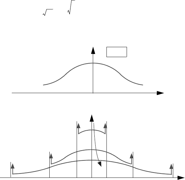
Next, we will examine various limits of the problem’s solution (7.474).

The limit leaves only

(7.476)

The field, initially located at the origin, travels in equal halves in the positive and

the negative z-direction. The reason for this even split is found in the initial

conditions (7.468) and (7.469). In case of different initial conditions, the field

would split in a different manner into the left and right travelling field (wave). In

any case, both fractions will move without changing their shape. The reason is that

these are ordinary plane waves travelling inside an ideal insulator (dielectric), as

outlined in Sect. 7.1.2 and they behave exactly as expected. Of course, the

separation into left and right travelling parts is possible in an arbitrary manner and

is specified by the initial conditions. Fig. 7.40 illustrates this motion. It is possible

to study the limit of pure diffusion. To achieve this, one lets in eq. (7.474),

or what amounts to the same, let . By means of the asymptotic formula

(3.181) for and , one obtains

(7.477)

which would also result from (6.78) when letting . In this case,

the field spreads to an increasingly widening Gaussian curve (Fig. 7.41). By this,

one has found both limiting cases (Fig. 7.40 and Fig. 7.41) from the general

solution. The general case is given by damped δ-functions travelling left and right

with the speed of light. There is no field in front of them. However, they drag an

Hct x–()

1for ct– xct<<

0for

xct –<

x +ct .>

















κ 0=

xt,()

---

δ xct–()δxct+()+[]=

Fig. 7.40

κ 0=

x()

-ct

ε 0→

c ∞→

xt,() F

µκ

4πt

--------

µκx

------------

–exp=

() Fδ x

()=

502 Time Dependent Problems II (Electromagnetic Waves)

umbrella of a diffusion field behind them. Fig. 7.42 illustrates this combination of

diffusion and wave propagation. One could say that it describes a compromise of

the trend shown in Figs. (7.40) and (7.41).

Although it would have been useful for practical reasons, to carry out these

calculations with dimensionless quantities, we have refrained from doing so here

(in contrast to the derivations of Sect. 6.4). This allowed to keep the dependency on

quantities with dimensions like, for example, ε and κ immediately visible, which

simplifies the limiting process. If one wants to save writing by use of

dimensionless quantities, the best way to proceed is this:

(7.478)

, (7.479)

with

(7.480)

, (7.481)

from which we can derive the wave equation as

Fig. 7.41

ε 0=

x()

Fig. 7.42

x()

x/ct

1-1 48-4-8

1.0

4.0

---=

8.0

---=

-----=

---=

κεµ

--------------

---

---== =

7.12 Boundary and Initial Value Problems 503

(7.482)

As a, so-to-speak, natural unit of time, we see the relaxation time , and as a

natural unit of the length, we take the distance through which light travels during

this time.

The Fourier transformation is another very useful tool to solve problems of

the kind discussed here. This solution decomposes the initial field (wave packet)

into its Fourier components. The previously discussed dispersion relation (Sect.

7.2) defines the behavior of each of these components, which allows the

superposition of these packets at a later time. We will not discuss this method here,

but it is nicely presented in detail in [8].

7.12.2 The Boundary Value Problem of the Half-Space

We shall revisit the problem of Sect. 6.5. Again, the task is to solve the wave

equation

(7.483)

now, however, in the half space with the boundary conditions:

(7.484)

(7.485)

and the initial conditions:

(7.486)

. (7.487)

The problem we have solved in Sect 6.5 was more general with respect to the initial

conditions. Conversely, there, we had one initial condition less. Using the Laplace

transform on eq. (7.483) gives:

(7.488)

while the boundary conditions in the p-domain become

(7.489)

. (7.490)

For the solution we obtain

(7.491)

Now, we choose

∂

ξτ,()

∂ξ

-------------------------

∂B

ξτ,()

∂τ

----------------------–

∂

ξτ,()

∂τ

-------------------------–0=

∂

∂x

----------- µκ

∂B

∂t

---------

– µε

∂

∂t

-----------

–0=

x 0>

∞ t,()finite=

0 t,() ft()=

x 0,()0=

∂B

xt,()

∂t

---------------------

t 0=

∂

xp,()

∂x

------------------------- µκp µεp

+()B

xp,()=

∞ p,()finite=

0 p,()f

p()=

xp,()f

p() µκp µεp

+– x[]exp=