Lehner G. Electromagnetic Field Theory for Engineers and Physicists

Подождите немного. Документ загружается.

504 Time Dependent Problems II (Electromagnetic Waves)

(7.492)

which results in

(7.493)

and therefore

(7.494)

The inverse Laplace transformation yields:

(7.495)

Here again, the best approach to prove this is by the transform of

according to eq. (7.495). We achieve this by using for example, [5], Vol. I, p. 200,

equation (8), and p. 129, eq. (5), which is the previously mentioned “damping

theorem”.

Specifically gives

(7.496)

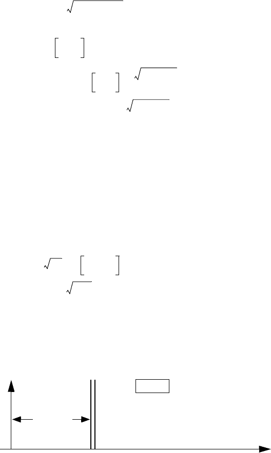
that is, the field of the very narrow impulse, created on the surface at

penetrates the medium with the speed of light. (Fig. 7.43). Conversely, if ,

then taking the limit and by means of eq. (3.181) one obtains

(7.497)

that is, just the result obtained when using eq. (6.111) and eq. (7.492). This

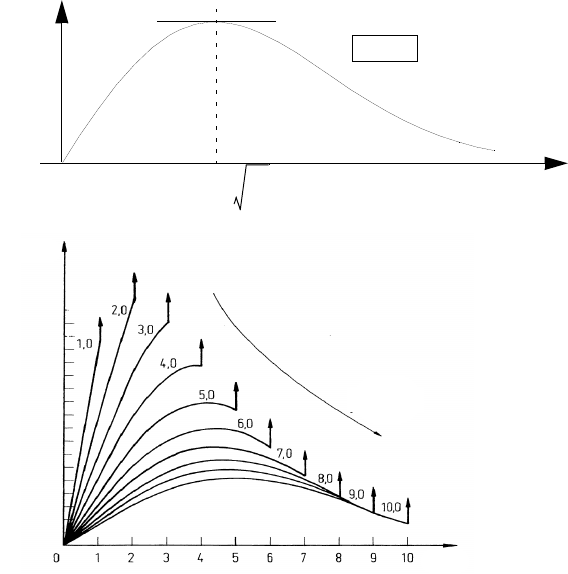
corresponds to a pure diffusion process (Fig. 7.44).

The general case involves a damped δ-function and a diffusing field, which

the δ-function drags behind itself. There is no field in front of the δ-function.

t() Gδ t()=

p() G=

xp,()G µκp µεp

+– x[]exp=

xt,() G

κx

2εc

---------–exp δ t

--–





κx

κt

2ε

-----– exp I

–

2εc

-------------------------





–





2ε c

–

--------------------------------------------------------------------------------------------

xt,()

κ 0=

xt,() Gδ t

--–





t 0=

Fig. 7.43

x()

xct=

κ 0=

ε 0=

xt,() G

x µκ

µκx

------------– exp

4πt

-----------------------------------------------

7.12 Boundary and Initial Value Problems 505

Various states of this process are illustrated in Fig. 7.45. For times , the field

looks more and more like the one shown in Fig. 7.44

Fig. 7.44

x()

max

µκ

-------=

ε 0=

Fig. 7.45

x()

x/ct

---=

t 4t

8 Numerical Methods

8.1 Introduction

This text has introduced the terminology of electromagnetic field theory, which

governs the relations between the various field quantities – Maxwell’s equations in

particular – and a few of the methods that are suitable to analytically solve field

theoretical problems. It is obvious, however, that for many problems, analytical

methods may only allow for an approximate solution or may not be solvable this

way at all. If we need to solve such problems, a different methodology has to be

employed. Sometimes, if the problem under consideration differs only slightly

from one that can be solved exactly, then perturbation theory may be applied. We

shall not discuss perturbation in this text. A discussion of that topic can be found at

Morse Feshbach [9]. In contrast, the various types of numerical methods are

generally applicable, at least in principle. In light of the ever increasing potential of

computer power, these methods become more and more attractive and constitute a

fruitful area for field theory as well. The subject is so vast, that we can only touch

on the basic ideas. On the other hand, numerical methods are so important that it

should not go unmentioned and therefore, the following shall be dedicated to

describe the most important numerical methods, including some simple examples.

Although we will focus on electrostatic problems, these methods are applicable to

all areas of field theory, in particular to magnetostatics and to time dependent

problems. It shall particularly be illustrated that, and how the various methods

relate to the analytical methods formally, and in to the field theoretical problems

from a content perspective. It is advisable to always work numerical and analytical

problems in parallel. This is an important basis for successful work in this area of

study. Such approach fosters a deeper and clearer understanding that is sufficiently

critical of the problem and its results. Areas for possible errors can be recognized

more easily and testing of the created programs can focus on the critical aspects of

the problem and thus be more efficient.

The following sections (8.2 though 8.5) prepare for the later sections (8.6

though 8.10), where the various numerical methods shall be explained.

8.2 Basics of Potential Theory

8.2.1 Boundary Value Problems and Integral Equations

The potential theory only briefly described in Sect. 3.4, is a basic building block for

both, the analytic as well as the numerical methods. This is particularly true for

Kirchhoff’s theorem (see 3.4.7, eq. (3.57)), which because of its far reaching

significance could easily be called the principal theorem of potential theory.

G. Lehner, Electromagnetic Field Theory for Engineers and Physicists,

DOI 10.1007/978-3-540-76306-2_8, © Springer-Verlag Berlin Heidelberg 2010

8.2 Basics of Potential Theory 507

(8.1)

This equation is valid for the three-dimensional space, where it addresses a point

inside a given region. We have already emphasized that the equation in this form is

not suitable to solve boundary values problems by arbitrarily specifying and

on the surface so that inside could be found. Only one or the other

boundary condition is allowed on any one surface element (in case of a mixed

boundary value problem, it has to be clear for which part of the area and for

which part applies. Nevertheless, we may use this equation to solve

boundary value problems (analytically, as well as numerically). Instead of using

eq. (8.1), for points on the surface one has

(8.2)

is a factor that for objects with smooth surfaces everywhere has a constant

value of . These are characterized by tangential planes which are uniquely

defined everywhere. For instance, the surface of a sphere is smooth. However, this

is not true for the surface of a cube (which has edges where it is obviously not

smooth), or that of a cone (which has a tip). Consider the three-dimensional δ-

function as the limit of a series of functions, which, within a given volume V, takes

on the constant value and vanishes outside of the volume. This makes it

intuitively clear that the integral necessary for the derivation of eq. (8.1), and of

eq. (3.57) in Sect. 3.4.7 becomes

where is the solid angle that arises at point of the surface inside the region.

For smooth surfaces, we have . On the edges of a cube the relation is

and at its corners . This allows one to include the

singular points of not-smooth surfaces as well.

A similar approach is possible for two-dimensional (plane) problems. In this

case, the so-called fundamental solution of the three-dimensional space

(8.3)

that is, the Coulomb potential of a point charge, has to be replaced by its two-

dimensional analogue, which is the potential of an infinitely long, straight, and

uniform line charge. Disregarding constant factors this is given by

(8.4)

where

(8.5)

With this, instead of eq. (8.1), we obtain for points inside a two-dimensional region

4πϕ r()

ρ r'()τ'd

rr'–

--------------------

∫

rr'–

---------------

∫

n'∂

∂

ϕ r'()dA' ϕ r'()

n'∂

∂ 1

rr'–

---------------dA'

∫

–+=

∂ϕ ∂n⁄ϕ

∂ϕ ∂n⁄

C r()ϕr()

ρ r'()τ'd

rr'–

--------------------

∫

rr'–

---------------

∫

∂ϕ r'()

∂n'

---------------

dA' ϕ r'()

n'∂

∂ 1

rr'–

---------------dA'

∫

–+=

C r()

2π

1 V⁄

ϕ r()4πδ rr'–()τd

∫

C r'()ϕr'() Ωϕr'()==

Ω r'

C 2π=

C Ωπ== C Ωπ2⁄==

rr'–

---------------=

ψ rr'–ln–=

∇

rr'–ln 2πδ rr'–() =

508 Numerical Methods

(8.6)

The last two integrals are line integrals along the path element which

constitutes the boundary of the area. On the boundary itself one has

(8.7)

The quantities and in equations (8.4) through (8.7) are two-dimensional

vectors in a plane.

represents the plane angle seen from inside the area. In case of a

smooth boundary, , for the corners of a rectangle we have , etc.

In case of one-dimensional problems, the fundamental solution can be

expressed in the form

(8.8)

This case yields

(8.9)

and by Sect. 3.4.5

(8.10)

The discontinuity of at is typical and of immense significance. This is

similar to the discontinuities of or in case

of three- or two dimensions, respectively. The value of the function at location

is the average of the left and right sided limit at this point.

If one wishes to solve a Dirichlet or Neumann boundary value problem, to

start with eq. (8.2) or eq. (8.7) is advisable in order to find the boundary values of

from those of or vice versa. This method provides compatible values for

and over the entire boundary. With these, eq. (8.1) or eq. (8.6) finally

allow one to determine the potential in the entire region. The boundary value

problem is thereby reduced to these integral equations.

If, in case of a Dirichlet problem, is given, then eq. (8.2) or eq. (8.7)

represent the so-called Fredholm Integral equation of the 1st kind for . In

2πϕ r()

ρ r'()

------------

rr'–ln A'd

∫

– rr'–ln

∫

∂ϕ r'()

∂n'

---------------

ds'+ ϕ r'()

n'∂

∂

rr'–ln ds'

∫

–=

ds'

C r()ϕr()

ρ r'()

------------

rr'–ln A'd

∫

– rr'–ln

∫

∂ϕ r'()

∂n'

---------------

ds'–=

ϕ r'()

n'∂

∂

rr'–ln ds'

∫

rr'

C r()

C π= C π 2⁄=

ψ xx',()

---

xx'–

---

x' x–() for xx' ≤

---

xx'–() for xx' .≥











ψ'

x∂

∂

---–forxx'<

0 for xx'=

---

for xx'>





















---– Hx x'–()+== =

ψ'' ∇

ψδxx'–()==

ψ' xx'=

∂∂n'⁄()1 rr'–⁄()

∂∂n'⁄()rr'–ln()

ψ'

xx'=

∂ϕ ∂n⁄ϕ

∂ϕ ∂n⁄

8.2 Basics of Potential Theory 509

case of a Neumann problem, eq. (8.2) or eq. (8.7) represent the Fredholm Integral

equation of the 2nd kind for .

There is another way how boundary value problems can be reduced to

integral equations. Consider a surface bounding a region carrying a surface charge

density . Then in the three-dimensional case (the one- and two-dimensional

cases can be solved analogously), the potential inside the volume and on the

boundary is

(8.11)

The perpendicular component of the electric field is discontinuous at the surface, as

we have already discovered before (Sect. 2.5.3 and 2.10). On the inside of the

surface, it is therefore

(8.12)

If there is a double layer or dipole layer on the surface with the surface density of

the dipole moment , then the potential is

(8.13)

In this case, even is discontinuous at the surface (see Sect. 2.5.3, eq. (2.73),

eq. (2.82)). The potential on the inside of the double layer is

(8.14)

From a formal perspective, both discontinuities are a consequence of the fact that

is discontinuous on the surface. Eqs (8.12) and (8.14) are valid

for an approach of the surface from the inside, in order to calculate the surface

integrals. The additional terms of Eqs (8.12) and (8.14) carry a factor 1/2, which is

a result of the fact that the value on the surface is obtained as an average of the both

sided limit, which can be regarded as dividing the discontinuities and

in half.

Eqs. (8.11) through (8.14) may be used to calculate the solutions of Dirichlet,

Neumann, or mixed boundary value problems. We start by just considering points

on the boundary. For Dirichlet problems, one finds either from (8.11) or

from (8.14). From there, either use (8.11) or (8.13) to find the potential in the

entire region. In case of Neumann problems, one calculates by means of

(8.12) and then finds the potential in the entire region by (8.11). Again, depending

on the type of problem, one needs to solve either the Fredholm Integral equations

of the 1st or 2nd kind.

These integral equations are of fundamental significance for field theory. For

the Fredholm Integral equations, there exists a well established mathematical

theory, which is also plausible because it is entirely analogous to the theory of

linear algebraic equations. The Fredholm Integral equations are nothing else than

σ r()

ϕ r()

σ r'()

4πε

rr'–

---------------------------

dA'

∫

∂ϕ r()

∂n

--------------

σ r'()

4πε

------------

∂

∂n

------

rr'–

---------------

dA'

∫

σ r()

2ε

-----------

ϕ r()

τ r()

4πε

------------

∂

∂n'

-------

rr'–

---------------

dA'

∫

ϕ r()

τ r'()

4πε

------------

∂

∂n'

-------

rr'–

---------------

dA'

∫

τ r()

2ε

----------

–=

∂∂n'⁄()1 rr'–⁄()

σε

⁄τε

⁄

σ r'()

τ r'()

σ r'()

510 Numerical Methods

the continuum analogues of linear algebraic equations. For instance, there are

theorems about the existence or non-existence of solutions, as well as their

uniqueness or multiplicity, which are an almost verbatim copy of their analogue in

linear systems of equations. They form the basis for many fundamental theorems of

potential theory, for example about the existence of solutions of boundary value

problems (see for example [10 through 16]). An analytical solution of the equations

is possible in some cases, which is what shall be demonstrated in the following by

an example. Finally – and this is important for our case – they are also suitable for

numerical evaluation, which results in the boundary element method and is

presented in Sect 8.8.

8.2.2 Examples

8.2.2.1 The One-dimensional Problem

This basic problem illustrates how to use eqs (8.1) through (8.7) in the not so trivial

2-D and 3D cases. We use Green’s integral theorem in one-dimension

(8.15)

and let be according to eq. (8.10). Then we find for points inside

(8.16)

and on the surface (i.e. for or )

(8.17)

The factor corresponds to the factors or in eqs (8.2) and

(8.7), respectively.

We chose a simple example where

, ,

(8.18)

and the Dirichlet boundary conditions

(8.19)

The exact solution to this problem is

(8.20)

This solution shall be obtained by means of the one-dimensional Kirchhoff

theorem, eqs. (8.16) and (8.17). We start from eq. (8.18) with eq. (8.8)

(8.21)

From eq. (8.17), and the fact that the surface consists of only two points, it follows

that

ψϕ'' ϕψ''–()xd

∫

ψϕ' ϕψ'–[]

ψ''

ϕ x'() ψ∇

ϕ xd

∫

ϕψ' ψϕ'–[]

+= ax' b<<

x' a= x' b=

---

ϕ x'() ψ∇

ϕ xd

∫

ϕψ' ψϕ'–[]

12⁄ C 2π= C π=

∇

ϕ Ax=0x 1≤≤

ϕ 0() ϕ1() 0==

Ax x

1–()

--------------------------=

ψ∇

ϕ xd

∫

------

2x'

3x'–2+()=

8.2 Basics of Potential Theory 511

with the solutions

, .

(8.22)

Thereby, the boundary values of determine the boundary values of (the

perpendicular derivatives). Together with eq. (8.16), they provide the solution

which is the same as previously given in eq. (8.20).

As our second example we choose

, ,

(8.23)

where

, .

(8.24)

Again, using eq. (8.17) gives

Note that here, is discontinuous for and by eq. (8.9)

, .

Furthermore:

and

This means that by eq. (8.16)

---

ϕ 0() 0

--- ψ 10,()ϕ'1() ψ00,()ϕ'0()–[]–==

---

ϕ 1() 0

------ ψ 11,()ϕ'1() ψ01,()ϕ'0()–[]–==

---

ϕ'1()⋅ 0 ϕ'0()⋅–=

------0ϕ'1()⋅

---

ϕ'0()⋅–=

ϕ'0()

---–= ϕ'1()

---=

ϕ∂ϕ∂n⁄

ϕ x'()

------

2x'

3x'–2+()

---

1 x'–

------------

⋅

---

⋅––

Ax' x'

1–()

----------------------------==

∇

ϕ 0=0x 1≤≤

ϕ 0() A= ϕ 1() B=

---

ϕ 0()

--- Bψ'10,()Aψ'00,()– ϕ'1()ψ10,()– ϕ'0()ψ00,()+[]==

---

ϕ 1()

--- Bψ'11,()Aψ'01,()– ϕ'1()ψ11,()– ϕ'0()ψ01,()+[]==

ψ' xx',() xx'=

ψ'00,()0= ψ'11,()0=

---

ϕ'1()

------------–=

---

ϕ'0()

------------+=

ϕ'0() ϕ'1() BA–==

512 Numerical Methods

(8.25)

Of course, we obtain the linear potential, necessary for this case.

It shall be noted that the fundamental solution can be chosen differently.

Important is only that it satisfies eq. (8.10). Therefore, the function

with

can also be chosen as the fundamental solution. Naturally, both of our examples

will give the same result, which to verify is left for the reader as an exercise.

8.2.2.2 Dirichlet’s Boundary Value Problem of a Sphere

In this example, we will use the above presented integral equations to solve the

inner Dirichlet boundary value problem of a sphere, for which Laplace’s equation

holds (that is no charges) in three different ways. This requires an expansion of the

fundamental solution (i.e. the inverse distance) by means of spherical harmonics.

By eq. (3.324) we write

(8.26)

The upper term is valid for , while the lower one holds for . The

perpendicular gradient is

ϕ x'()

--- BA–()

1 x'–

------------

–

--- BA–()

---

++=

ABA–()x'+=

ψ xx',()

x'1 x+() for xx'≤

x 1 x'+() for xx'≥







ψ' xx',()

∂ψ

∂x

-------

x' for xx'<

--- x'+ for xx'=

1 x'+ for xx'>





















x' Hx x'–()+== =

–

---------------- 2 δ

–()

n 1+

------------

n 1+

------------











m 0=

∑

n 0=

∞

∑

nm–()!

nm+()!

--------------------

P⋅

θcos()P

cos()m ϕϕ

–()[]cos

≤ rr

≥

8.2 Basics of Potential Theory 513

(8.27)

Significant is that the expression is discontinuous for . Now, the upper term

is valid for , the middle term is for , and the lower one holds for

. This discontinuity is the main reason for presenting this example here.

From a formal perspective, this is the reason for the discontinuity of the electric

field at charged surfaces and that of the potential at dipole layers which was

demonstrated in Sect. 2.5.3 and has culminated in the integrals eq. (8.12) and

eq. (8.14). This shall be demonstrated again by means of the present example. Note

the frequently used relation:

We also need the completeness relation for the spherical harmonics. It results form

expanding in terms of spherical harmonics by means of

eq. (3.300) and the corresponding expression, now using sine instead of cosine:

We start by analyzing the integral in eq. (8.12). With the exception of the sign, the

perpendicular gradient contained therein is given by eq. (8.27). For we find

that at the inside and the outside boundary, respectively:

∂

∂n

--------

–

----------------

2 δ

–()

n 1+()

n 2+

------------

–

--------–

n 1–

n 1+

------------











m 0=

∑

n 0=

∞

∑

nm–()!

nm+()!

--------------------

P⋅

θcos()P

cos()m ϕϕ

–()[]cos

< rr

∂

∂n

------

rr'–

---------------

∂

∂n'

-------

rr'–

---------------

–=

δθ θ'–()δϕϕ'–()

2n 1+()nm–()!

4π nm+()!

-----------------------------------------

2 δ

–()

m 0=

∑

n 0=

∞

∑

θcos()P

θ'cos()m ϕϕ'–()[]cos θ'sin

δθ θ'–()δϕϕ'–()=

∂

∂n'

-------

rr'–

---------------

nm–()!

nm+()!

--------------------

2 δ

–()P

θcos()P

θ'cos()

m 0=

∑

n 0=

∞

∑

–=

m ϕϕ'–()[]cos

n 1+()–

--------------------

-----











⋅