Manning Ch. D., Raghavan P., Sch?tze H. Introduction to Information Retrieval - Введение в информационный поиск

Подождите немного. Документ загружается.

Online edition (c)2009 Cambridge UP

316 14 Vector space classiﬁcation

0 1 2 3 4 5 6 7 8

◮

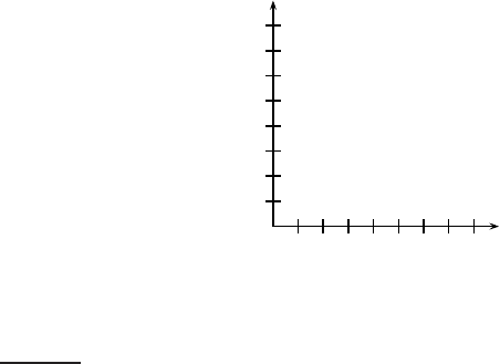
Figure 14.14 Example for differences between Euclidean distance, dot product

similarity and cosine similarity. The vectors are ~a = (0.5 1.5)

, ~x = (2 2)

b =

(4 4)

, and~c = (8 6)

plement Rocchio classiﬁcation and kNN classiﬁcation, for example, the Bow toolkit

(McCallum 1996).

Exercise 14.8

Download 20 Newgroups (page 154) and train and test Rocchio and kNN classiﬁers

for its 20 classes.

Exercise 14.9

Show that the decision boundaries in Rocchio classiﬁcation are, as in kNN, given by

the Voronoi tessellation.

Exercise 14.10 [⋆]

Computing the distance between a dense centroid and a sparse vector is Θ(M) for

a naive implementation that iterates over all M dimensions. Based on the equality

∑

− µ

)

= 1.0 +

∑

−2

∑

and assuming that

∑

has been precomputed,

write down an algorithm that is Θ(M

) instead, where M

is the number of distinct

terms in the test document.

Exercise 14.11 [⋆ ⋆ ⋆]

Prove that the region of the plane consisting of all points with the same k nearest

neighbors is a convex polygon.

Exercise 14.12

Design an algorithm that performs an efﬁcient 1NN search in 1 dimension (where

efﬁciency is with respect to the number of documents N). What is the time complexity

of the algorithm?

Exercise 14.13 [⋆ ⋆ ⋆]

Design an algorithm that performs an efﬁcient 1NN search in 2 dimensions with at

most polynomial (in N) preprocessing time.

Online edition (c)2009 Cambridge UP

14.8 Exercises 317

◮

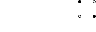
Figure 14.15 A simple non-separable set of points.

Exercise 14.14 [⋆ ⋆ ⋆]

Can one design an exact efﬁcient algorithm for 1NN for very large M along the ideas

you used to solve the last exercise?

Exercise 14.15

Show that Equation (14.4) deﬁnes a hyperplane with ~w = ~µ(c

) −~µ(c

) and b =

0.5 ∗ (|~µ(c

−|~µ(c

Exercise 14.16

We can easily construct non-separable data sets in high dimensions by embedding

a non-separable set like the one shown in Figure

14.15. Consider embedding Fig-

ure

14.15 in 3D and then perturbing the 4 points slightly (i.e., moving them a small

distance in a random direction). Why would you expect the resulting conﬁguration

to be linearly separable? How likely is then a non-separable set of m ≪ M points in

M-dimensional space?

Exercise 14.17

Assuming two classes, show that the percentage of non-separable assignments of the

vertices of a hypercube decreases with dimensionality M for M > 1. For example,

for M = 1 the proportion of non-separable assignments is 0, for M = 2, it is 2/16.

One of the two non-separable cases for M = 2 is shown in Figure

14.15, the other is

its mirror image. Solve the exercise either analytically or by simulation.

Exercise 14.18

Although we point out the similarities of Naive Bayes with linear vector space classi-

ﬁers, it does not make sense to represent count vectors (the document representations

in NB) in a continuous vector space. There is however a formalization of NB that is

analogous to Rocchio. Show that NB assigns a document to the class (represented as

a parameter vector) whose Kullback-Leibler (KL) divergence (Section

12.4, page 251)

to the document (represented as a count vector as in Section

13.4.1 (page 270), nor-

malized to sum to 1) is smallest.

Online edition (c)2009 Cambridge UP

DRAFT! © April 1, 2009 Cambridge University Press. Feedback welcome. 319

Support vector machines and

machine learni ng on d ocuments

Improving classiﬁer effectiveness has been an area of intensive machine-

learning research over the last two decades, and this work has led to a new

generation of state-of-the-art classiﬁers, such as support vector machines,

boosted decision trees, regularized logistic regression, neural networks, and

random forests. Many of these methods, including support vector machines

(SVMs), the main topic of this chapter, have been applied with success to

information retrieval problems, particularly text classiﬁcation. An SVM is a

kind of large-margin classiﬁer: it is a vector space based machine learning

method where the goal is to ﬁnd a decision boundary between two classes

that is maximally far from any point in the training data (possibly discount-

ing some points as outliers or noise).

We will initially motivate and develop SVMs for the case of two-class data

sets that are separable by a linear classiﬁer (Section 15.1), and then extend the

model in Section

15.2 to non-separable data, multi-class problems, and non-

linear models, and also present some additional discussion of SVM perfor-

mance. The chapter then moves to consider the practical deployment of text

classiﬁers in Section

15.3: what sorts of classiﬁers are appropriate when, and

how can you exploit domain-speciﬁc text features in classiﬁcation? Finally,

we will consider how the machine learning technology that we have been

building for text classiﬁcation can be applied back to the problem of learning

how to rank documents in ad hoc retrieval (Section

15.4). While several ma-

chine learning methods have been applied to this task, use of SVMs has been

prominent. Support vector machines are not necessarily better than other

machine learning methods (except perhaps in situations with little training

data), but they perform at the state-of-the-art level and have much current

theoretical and empirical appeal.

Online edition (c)2009 Cambridge UP

320 15 Support vector machines and machine learning on documents

Support vectors

Maximum

margin

decision

hyperplane

Margin is

maximized

◮

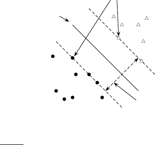
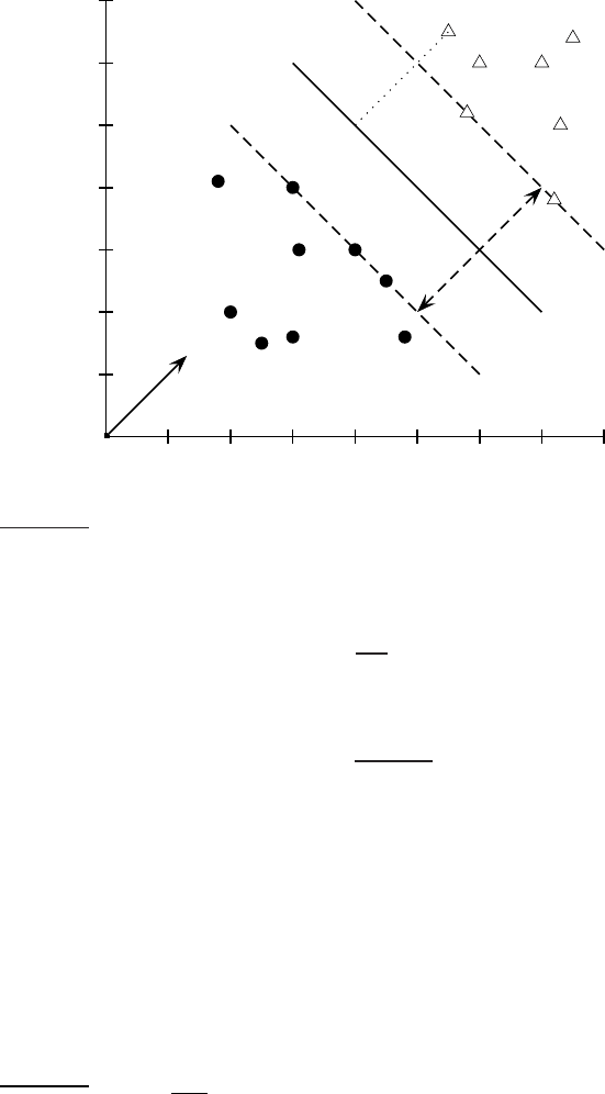
Figure 15.1 The support vectors are the 5 points right up against the margin of

the classiﬁer.

15.1 Supp ort vector machines: The linearly separable case

For two-class, separable training data sets, such as the one in Figure

14.8

(page 301), there are lots of possible linear separators. Intuitively, a decision

boundary drawn in the middle of the void between data items of the two

classes seems better than one which approaches very close to examples of

one or both classes. While some learning methods such as the perceptron

algorithm (see references in Section

14.7, page 314) ﬁnd just any linear sepa-

rator, others, like Naive Bayes, search for the best linear separator according

to some criterion. The SVM in particular deﬁnes the criterion to be looking

for a decision surface that is maximally far away from any data point. This

distance from the decision surface to the closest data point determines the

margin of the classiﬁer. This method of construction necessarily means thatMARGIN

the decision function for an SVM is fully speciﬁed by a (usually small) sub-

set of the data which deﬁnes the position of the separator. These points are

referred to as the support vectors (in a vector space, a point can be thought ofSUPPORT VECTOR

as a vector between the origin and that point). Figure

15.1 shows the margin

and support vectors for a sample problem. Other data points play no part in

determining the decision surface that is chosen.

Online edition (c)2009 Cambridge UP

15.1 Support vector machines: The linearly separable case 321

◮

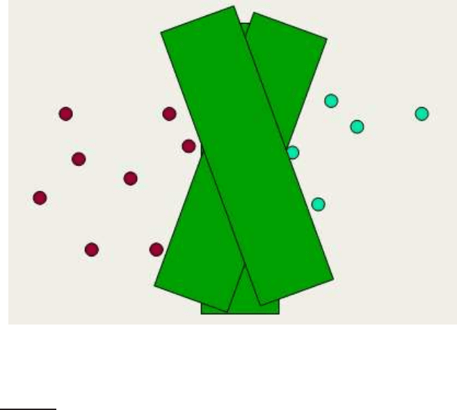
Figure 15.2 An intuition for large-margin classiﬁcation. Insisting on a large mar-

gin reduces the capacity of the model: the range of angles at which the fat deci-

sion surface can be placed is smaller than for a decision hyperplane (cf. Figure 14.8,

page 301).

Maximizing the margin seems good because points near the decision sur-

face represent very uncertain classiﬁcation decisions: there is almost a 50%

chance of the classiﬁer deciding either way. A classiﬁer with a large margin

makes no low certainty classiﬁcation decisions. This gives you a classiﬁca-

tion safety margin: a slight error in measurement or a slight document vari-

ation will not cause a misclassiﬁcation. Another intuition motivating SVMs

is shown in Figure

15.2. By construction, an SVM classiﬁer insists on a large

margin around the decision boundary. Compared to a decision hyperplane,

if you have to place a fat separator between classes, you have fewer choices

of where it can be put. As a result of this, the memory capacity of the model

has been decreased, and hence we expect that its ability to correctly general-

ize to test data is increased (cf. the discussion of the bias-variance tradeoff in

Chapter

14, page 312).

Let us formalize an SVM with algebra. A decision hyperplane (page 302)

can be deﬁned by an intercept term b and a decision hyperplane normal vec-

tor ~w which is perpendicular to the hyperplane. This vector is commonly

Online edition (c)2009 Cambridge UP

322 15 Support vector machines and machine learning on documents

referred to in the machine learning literature as the weight vector. To chooseWEIGHT VECTOR

among all the hyperplanes that are perpendicular to the normal vector, we

specify the intercept term b. Because the hyperplane is perpendicular to the

normal vector, all points ~x on the hyperplane satisfy ~w

~x = −b. Now sup-

pose that we have a set of training data points D = {(~x

, y

)}, where each

member is a pair of a point ~x

and a class label y

corresponding to it.

For

SVMs, the two data classes are always named +1 and −1 (rather than 1 and

0), and the intercept term is always explicitly represented as b (rather than

being folded into the weight vector ~w by adding an extra always-on feature).

The math works out much more cleanly if you do things this way, as we will

see almost immediately in the deﬁnition of functional margin. The linear

classiﬁer is then:

f (~x) = sign(~w

~x + b)

(15.1)

A value of −1 indicates one class, and a value of +1 the other class.

We are conﬁdent in the classiﬁcation of a point if it is far away from the

decision boundary. For a given data set and decision hyperplane, we deﬁne

the functional margin of the i

example ~x

with respect to a hyperplane h~w, biFUNCTIONAL MARGIN

as the quantity y

(~w

+ b ). The functional margin of a data set with re-

spect to a decision surface is then twice the functional margin of any of the

points in the data set with minimal functional margin (the factor of 2 comes

from measuring across the whole width of the margin, as in Figure

15.3).

However, there is a problem with using this deﬁnition as is: the value is un-

derconstrained, because we can always make the functional margin as big

as we wish by simply scaling up ~w and b. For example, if we replace ~w by

5~w and b by 5b then the functional margin y

(5~w

+ 5b) is ﬁve times as

large. This suggests that we need to place some constraint on the size of the

~w vector. To get a sense of how to do that, let us look at the actual geometry.

What is the Euclidean distance from a point ~x to the decision boundary? In

Figure

15.3, we denote by r this distance. We know that the shortest distance

between a point and a hyperplane is perpendicular to the plane, and hence,

parallel to ~w. A unit vector in this direction is ~w/|~w|. The dotted line in the

diagram is then a translation of the vector r~w/|~w|. Let us label the point on

the hyperplane closest to ~x as ~x

′

. Then:

′

= ~x − yr

|~w|

(15.2)

where multiplying by y just changes the sign for the two cases of ~x being on

either side of the decision surface. Moreover,~x

′

lies on the decision boundary

1. As discussed in Section 14.1 (page 291), we present the general case of points in a vector

space, but if the points are length normalized document vectors, then all the action is taking

place on the surface of a unit sphere, and the decision surface intersects the sphere’s surface.

Online edition (c)2009 Cambridge UP

15.1 Support vector machines: The linearly separable case 323

0 1 2 3 4 5 6 7 8

′

◮

Figure 15.3 The geometric margin of a point (r) and a decision boundary (ρ).

and so satisﬁes ~w

′

+ b = 0. Hence:



~x −yr

|~w|



+ b = 0

(15.3)

Solving for r gives:

r = y

~x + b

|~w|

(15.4)

Again, the points closest to the separating hyperplane are support vectors.

The geometric m argin of the classiﬁer is the maximum width of the band thatGEOMETRIC MARGIN

can be drawn separating the support vectors of the two classes. That is, it is

twice the minimum value over data points for r given in Equation (

15.4), or,

equivalently, the maximal width of one of the fat separators shown in Fig-

ure

15.2. The geometric margin is clearly invariant to scaling of parameters:

if we replace ~w by 5~w and b by 5b, then the geometric margin is the same, be-

cause it is inherently normalized by the length of ~w. This means that we can

impose any scaling constraint we wish on ~w without affecting the geometric

margin. Among other choices, we could use unit vectors, as in Chapter

6, by

2. Recall that |~w| =

√

~w.

Online edition (c)2009 Cambridge UP

324 15 Support vector machines and machine learning on documents

requiring that |~w| = 1. This would have the effect of making the geometric

margin the same as the functional margin.

Since we can scale the functional margin as we please, for convenience in

solving large SVMs, let us choose to require that the functional margin of all

data points is at least 1 and that it is equal to 1 for at least one data vector.

That is, for all items in the data:

(~w

+ b) ≥ 1(15.5)

and there exist support vectors for which the inequality is an equality. Since

each example’s distance from the hyperplane is r

= y

(~w

+ b)/|~w|, the

geometric margin is ρ = 2/|~w|. Our desire is still to maximize this geometric

margin. That is, we want to ﬁnd ~w and b such that:

• ρ = 2/|~w| is maximized

• For all (~x

, y

) ∈ D, y

(~w

+ b) ≥ 1

Maximizing 2/|~w| is the same as minimizing |~w|/2. This gives the ﬁnal stan-

dard formulation of an SVM as a minimization problem:

(15.6) Find ~w and b such that:

•

~w is minimized, and

• for all {(~x

, y

)}, y

(~w

+ b) ≥ 1

We are now optimizing a quadratic function subject to linear constraints.

Quadratic optimiza tion problems are a standard, well-known class of mathe-QUADRATIC

PROGRAMMING

matical optimization problems, and many algorithms exist for solving them.

We could in principle build our SVM using standard quadratic programming

(QP) libraries, but there has been much recent research in this area aiming to

exploit the structure of the kind of QP that emerges from an SVM. As a result,

there are more intricate but much faster and more scalable libraries available

especially for building SVMs, which almost everyone uses to build models.

We will not present the details of such algorithms here.

However, it will be helpful to what follows to understand the shape of the

solution of such an optimization problem. The solution involves construct-

ing a dual problem where a Lagrange multiplier α

is associated with each

constraint y

(~w

+ b) ≥ 1 in the primal problem:

(15.7) Find α

, . . . α

such that

∑

−

∑

is maximized, and

•

∑

= 0

• α

≥ 0 for all 1 ≤ i ≤ N

The solution is then of the form:

Online edition (c)2009 Cambridge UP

15.1 Support vector machines: The linearly separable case 325

0 1 2 3

◮

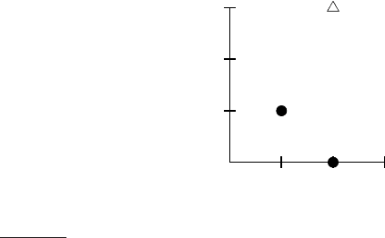
Figure 15.4 A tiny 3 data point training set for an SVM.

(15.8) ~w =

∑

b = y

− ~w

for any ~x

such that α

6= 0

In the solution, most of the α

are zero. Each non-zero α

indicates that the

corresponding ~x

is a support vector. The classiﬁcation function is then:

f (~x) = sign(

∑

~x + b)

(15.9)

Both the term to be maximized in the dual problem and the classifying func-

tion involve a dot product between pairs of points (~x and ~x

or ~x

and ~x

), and

that is the only way the data are used – we will return to the signiﬁcance of

this later.

To recap, we start with a training data set. The data set uniquely deﬁnes

the best separating hyperplane, and we feed the data through a quadratic

optimization procedure to ﬁnd this plane. Given a new point ~x to classify,

the classiﬁcation function f (~x) in either Equation (

15.1) or Equation (15.9) is

computing the projection of the point onto the hyperplane normal. The sign

of this function determines the class to assign to the point. If the point is

within the margin of the classiﬁer (or another conﬁdence threshold t that we

might have determined to minimize classiﬁcation mistakes) then the classi-

ﬁer can return “don’t know” rather than one of the two classes. The value

of f (~x) may also be transformed into a probability of classiﬁcation; ﬁtting

a sigmoid to transform the values is standard (Platt 2000). Also, since the

margin is constant, if the model includes dimensions from various sources,

careful rescaling of some dimensions may be required. However, this is not

a problem if our documents (points) are on the unit hypersphere.

✎

Example 15.1 : Consider building an SVM over the (very little) data set shown in

Figure

15.4. Working geometrically, for an example like this, the maximum margin

weight vector will be parallel to the shortest line connecting points of the two classes,

that is, the line between (1, 1) and (2, 3), giving a weight vector of (1, 2). The opti-

mal decision surface is orthogonal to that line and intersects it at the halfway point.