Marder M.P. Condensed Matter Physics

Подождите немного. Документ загружается.

Numerical Methods 273

then multiply the result by M again, and so on, repeatedly. The effect is to amplify

at an exponentially growing rate the component of a\ that is parallel to the lowest

eigenvector ê\. After multiplying a\ by M r times, the result is the vector

:êi{êi ·α\). Write a\ in a basis given by ê„ and begin mul- (10.15)

' «plying by M.

i=l

Because a\ has been chosen randomly, there is no reason for â-ê\ to vanish, and

as r grows, the term proportional to this factor must grow to dominate the sum.

The rapidity with which this happens depends upon the separation between λι and

\2',

if they are degenerate, then the first two terms in the sum grow together. In

any event, after sufficient multiplication of M upon a\, the result is proportional

to êi, and both the lowest eigenvector and eigenvalue are determined. What of the

next-lowest eigenvalue? It may be found by using the knowledge of ê\ to eliminate

anything proportional to ê\ from the sum (10.15). Repeat the multiplication pro-

cess,

but beginning with

cÎ2

= a\—ê\{ê\-a) rather than a\. If even a small bit of ë\

is left in the result due to numerical error, it will grow exponentially rapidly when

02 is multiplied by M. After every one or two multiplications one needs to project

out the component of

ë\

again. However, now the part of the sum dominated by the

next-lowest eigenvalue will grow exponentially out of all the rest, giving ëi. Given

êi, «3 =

0.2

—

êïiai

-ë-i),

provides a starting point for finding êj, and so on.

The task of multiplying an 800 x 800 matrix a few times into a vector is a great

improvement over the task of finding 800 eigenvalues, but is still burdensome. A

great virtue of using plane waves as basis functions lies in the fact that no matrix

of such a size needs to be stored at all, and its action upon wave vectors can be

computed much more rapidly than might at first seem possible.

Consider, for example, any Hamiltonian of the form

pi In order for this method to be effective, U should be a

ryr \-U (R\ P

seu

d°P

ote

ntial, smaller than the true ionic potential and ( i n I f.\

1™ \ )■ without a singularity near the origin. ^ ' '

The goal now is to find the lowest eigenvalues and corresponding eigenvectors of

Eq. (10.16), using the form of Schrödinger's equation displayed in Eq. (7.33) and

taking the wave function φ to have the form given in Eq. (7.35). Of course, instead

of using an infinite number of reciprocal lattice vectors, one builds ψ out of a finite

number of them. If the low-lying eigenvalues are to be deduced by multiplying ψ

repeatedly, one must begin by ensuring that the large negative eigenvalues of

Ji are larger in absolute value than the large positive eigenvalues. Suppose

max

to be the magnitude of the largest reciprocal lattice vector appearing in Eq. (7.33).

The kinetic energy of the corresponding plane wave would be /i

max

/2m = £

max

;

the kinetic energy dominates the large positive eigenvalues of "K, because the po-

tential energy of a plane wave with large

max

should be comparatively small. So,

taking the operator acting upon ψ to be

K' -,

This is a restatement of Eq. (7.33), with rp(q) written as V„j (K), where K is the reciprocal

lattice vector so that a

—

K = k lies in the first Brillouin zone.

274

Chapter 10. Realistic Calculations in Solids

one can now begin obtaining eigenvalues. The sum required to evaluate the poten-

tial energy seems to be numerically expensive, but in fact costs less than at first

appears. The action of the potential energy upon ψ is in the form of a convolution;

through use of the fast Fourier transform (Appendix A), J^,

U^^C^K')

can

be evaluated for Νχ values of K in only approximately Νκ In

operations, rather

than

as first appears.

Numerous variants of this basic method are possible. For example, instead of

multiplying the wave function by

"K,

one can multiply repeatedly by

l +

Mdt/h.

(10.18)

Thus one obtains eigenfunctions recursively from

■ψ

η+λ

= (l+ÎCdt/h)il>

ΨΧ+'-Ψ"

\<κ>ψ

(10.19)

dt h

which in the limit dt

—>

0 is a version of Schrödinger's equation with the time t

replaced by the imaginary quantity it. While electronic eigenfunctions are busy

iterating their way toward correct values, one can choose at the same time to allow

other features of the problem to vary. Most importantly, as progressively more

accurate wave functions are obtained, the charge density following from them must

be used to determine the terms dependent upon density in Eq. (9.104). In addition,

if the true equilibrium location of all atoms is not known, then at each iterative step

the forces on all atoms can be computed and the atoms can be allowed to move in

the directions of

the

forces. In this way, equilibrium atomic positions and electronic

wave functions can be computed simultaneously, as opposed to an approach in

which certain atomic positions are assumed, wave functions are calculated to high

accuracy, forces on atoms determined, the atoms moved, and the process begun

again. Car and Parrinello (1985) showed that it is possible to attempt dynamical

problems, in which ions move according to Newton's laws, driven by clouds of

electrons whose configurations are being calculated self-consistently while the ions

move.

10.2.4 Linear Augmented Plane Waves (LAPW)

All methods for solving the Schrödinger equation should in principle be the same.

However, numerical calculations for problems with an infinite number of degrees

of freedom are always approximate. Many methods aim to choose a set of basis

functions that approximate the real solutions as closely as possible, so that the de-

composition of true wave functions in terms of the basis with a small number of

terms has a hope of being accurate. Some of the most widely used are [linear]

augmented plane waves ([L]APW), Korringa-Kohn-Rostoker (KKR), and [linear]

muffin tin orbital ([L]MTO). These methods have many features in common with

each other, as well as with the plane wave method of the previous section, and

emphasize in varying degrees either the free-electron nature of electrons between

atoms or else the atomic nature of electrons near the cores. The codes with greatest

Numerical Methods 275

claim to accuracy tend to be expensive in terms of computational power and mem-

ory usage, while others making more severe approximations run faster on smaller

machines.

This section will briefly discuss augmented plane waves, which are due to

Slater (1937). The starting point is the observation after Eq. (7.47) that Bloch's

theorem provides the possibility of finding wave functions for the entire crystal by

solving Schrödinger's equation within a single unit cell, subject to the boundary

conditions recorded in Eq. (7.49).

In order to make the computation of boundary conditions simple, it is conven-

tional to mangle the periodic potential even beyond the point to which it has been

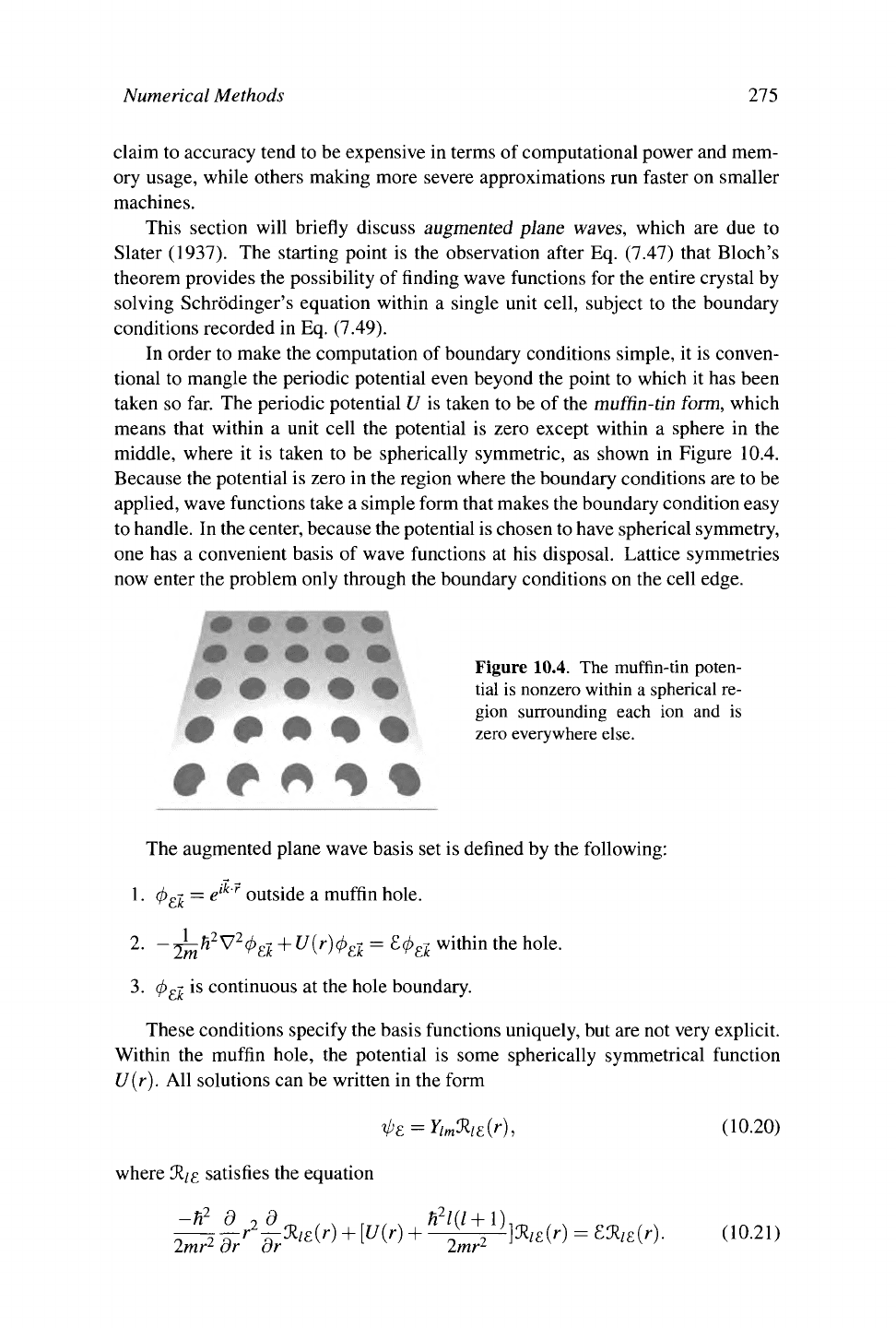
taken so far. The periodic potential U is taken to be of the muffin-tin form, which

means that within a unit cell the potential is zero except within a sphere in the

middle, where it is taken to be spherically symmetric, as shown in Figure 10.4.

Because the potential is zero in the region where the boundary conditions are to be

applied, wave functions take a simple form that makes the boundary condition easy

to handle. In the center, because the potential is chosen to have spherical symmetry,

one has a convenient basis of wave functions at his disposal. Lattice symmetries

now enter the problem only through the boundary conditions on the cell edge.

Figure 10.4. The muffin-tin poten-

tial is nonzero within a spherical re-

gion surrounding each ion and is

zero everywhere else.

The augmented plane wave basis set is defined by the following:

φ^ =

lkr

outside a muffin hole.

-^-Η

ι + υ(Γ)φ

ι = Εφ^ within the hole.

^ is continuous at the hole boundary.

These conditions specify the basis functions uniquely, but are not very explicit.

Within the muffin hole, the potential is some spherically symmetrical function

U(r).

All solutions can be written in the form

#=^AW, (10.20)

where 3?/g satisfies the equation

h2 9

~Ji

(r) + [U(r) + ^+H]

K/e

(r) = £K

/£

(r). (10.21)

2mr

dr dr 2mr

276 Chapter 10. Realistic Calculations in Solids

For an arbitrary £ there are two independent solutions to this equation, one of

which diverges at the origin, while the other diverges at infinity. One must discard

the solution that diverges at the origin, but divergences at infinity are of

concern,

because the solution need remain finite no further than the edge of the unit cell.

This second solution is therefore perfectly acceptable, and one can write

oo /

Φεί

= Σ Σ

(r)%

(r),

(10.22)

/=0 m=-/

where for the moment all of

the

coefficients

A.\

are arbitrary. They may be fixed by

application of the condition that the wave function be continuous across the muffin

hole boundary. Recall that

oo /

É^ = 47T^ J2

Jl(

)

lmC

)

lm(r)- See Landau and Lifshitz (1977), (10.23)

1=0 m=-l

Then, taking

R/,

to be the radius of the muffin hole, one has

♦"

^i«»UW).

00.24)

There is now a function φ for every £ and every k. The functions have a discontinu-

ity in slope at the muffin boundary, which there is not enough freedom to remove at

this stage. Next consider the problem of matching the boundary conditions (7.49)

at the edge of the primitive cell. Because the augmented plane waves are no more

than plane waves there, one can accomplish this task simply by considering func-

tions built to obey Bloch's theorem in the form

The K are reciprocal lattice vectors and

, g ( 10.25)

are coefficients to be determined. This ex-

pression is especially simple because of the

decision to set the potential U to zero outside

the muffin-tin.

The parameter £ is still allowed to vary freely. How should one think about it? The

augmented plane wave functions form a complete (not orthonormal) set for any £.

But one should only expect them to converge rapidly to a desired eigenfunction

by choosing £ to be the eigenvalue corresponding to that eigenfunction. Therefore,

during the numerical search for the coefficients

b^,

one should vary the parameter £

buried within the augmented plane wave functions so as to correspond to the latest

estimate of the eigenvalue and obtain the most rapid convergence of the series.

Although one need not set £ equal to the eigenvalue of Schrödinger's equation,

they often are the same, and they are denoted by the same symbol for this reason.

The only remaining task is to determine the coefficients b^,^. The best way

to do it is to use the variational principle of Eq. (B.l

1),

which directs one to insert

Eq. (10.25) into

(</>|A-£|V>), (10.26)

Ψϊ = Σ,

Η+κΦεΜκ-

Definition of Metals, Insulators, and Semiconductors

277

and then require all variations with respect to each

g to vanish. Let q and a' be

any vectors differing from k by a reciprocal lattice vector K. The result is then that

ο =

Σ<^|Α-εμ^^,

(10.27)

where

(φ^

Ä - ε

ΦΕ? ) = (

- ε ) Ω%

+ Uff The final answer is given by

^ ' i ' 2/jj ^'

^" diagonahzing this matrix.

the

volume of the unit

cell.

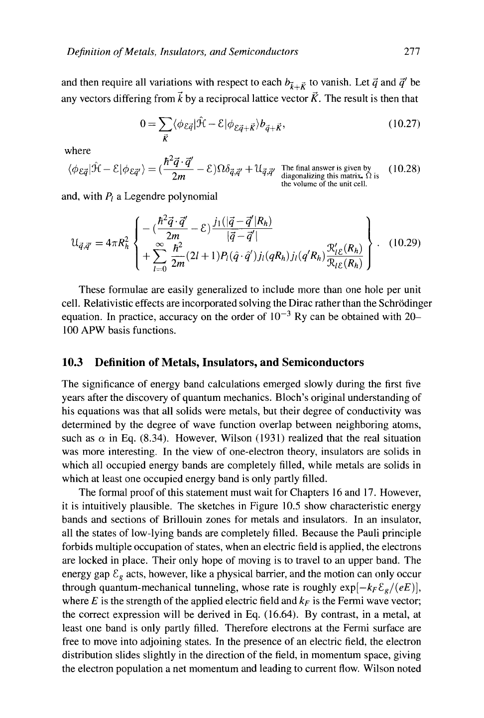
and, with P; a Legendre polynomial

= 4TTRI {

q-q'

gJ\{\q-q'\

\q-q

(10.28)

. (10.29)

These formulae are easily generalized to include more than one hole per unit

cell. Relativistic effects are incorporated solving the Dirac rather than the Schrödinger

equation. In practice, accuracy on the order of 10

-3

Ry can be obtained with 20-

100 APW basis functions.

10.3 Definition of Metals, Insulators, and Semiconductors

The significance of energy band calculations emerged slowly during the first five

years after the discovery of quantum mechanics. Bloch's original understanding of

his equations was that all solids were metals, but their degree of conductivity was

determined by the degree of wave function overlap between neighboring atoms,

such as Q in Eq. (8.34). However, Wilson (1931) realized that the real situation

was more interesting. In the view of one-electron theory, insulators are solids in

which all occupied energy bands are completely filled, while metals are solids in

which at least one occupied energy band is only partly filled.

The formal proof of this statement must wait for Chapters 16 and 17. However,

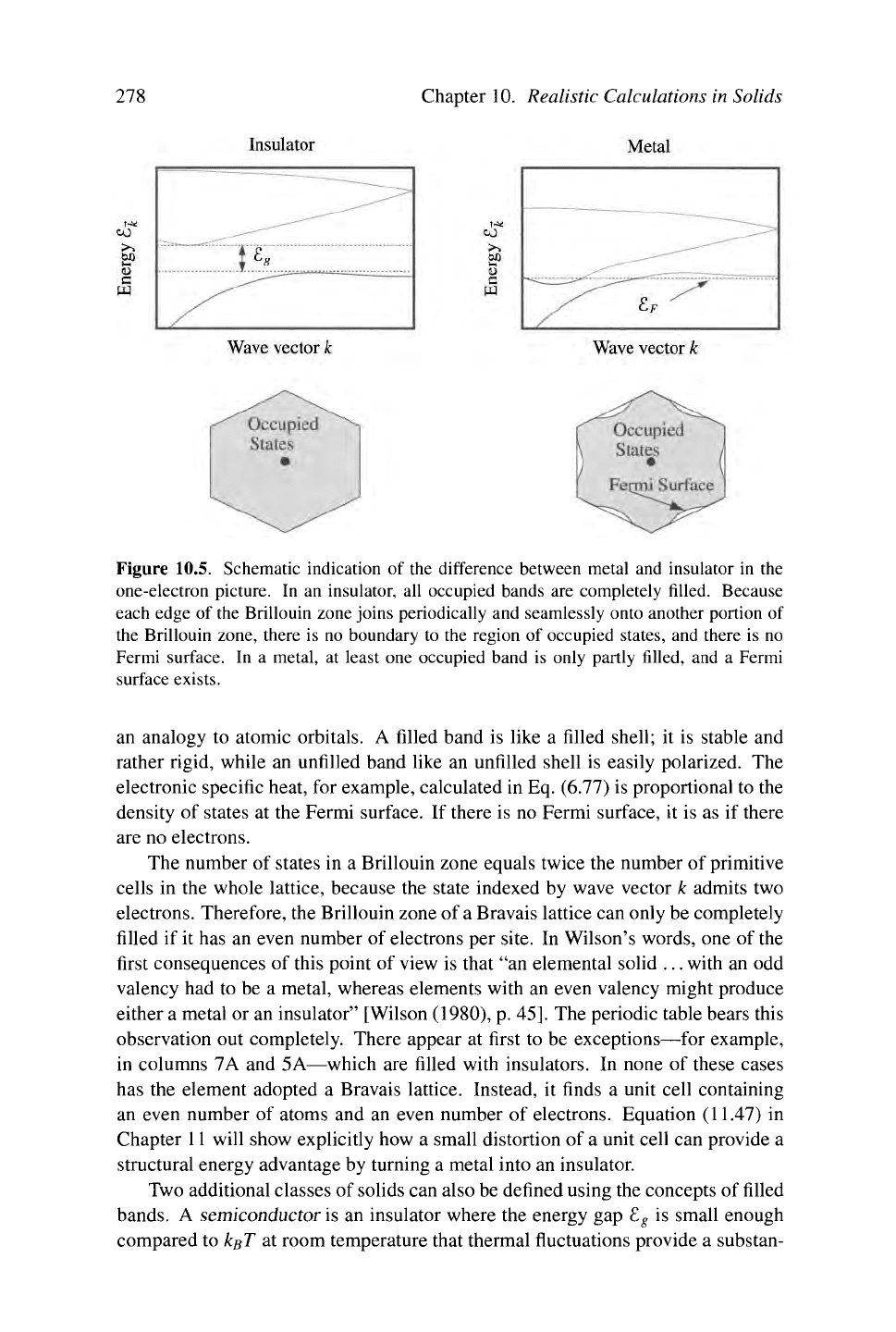
it is intuitively plausible. The sketches in Figure 10.5 show characteristic energy

bands and sections of Brillouin zones for metals and insulators. In an insulator,

all the states of low-lying bands are completely filled. Because the Pauli principle

forbids multiple occupation of

states,

when an electric field is applied, the electrons

are locked in place. Their only hope of moving is to travel to an upper band. The

energy gap E

acts, however, like a physical barrier, and the motion can only occur

through quantum-mechanical tunneling, whose rate is roughly exp[—kpE

/(eE)},

where E is the strength of

the

applied electric field and kp is the Fermi wave vector;

the correct expression will be derived in Eq. (16.64). By contrast, in a metal, at

least one band is only partly filled. Therefore electrons at the Fermi surface are

free to move into adjoining states. In the presence of an electric field, the electron

distribution slides slightly in the direction of the field, in momentum space, giving

the electron population a net momentum and leading to current flow. Wilson noted

278 Chapter 10. Realistic Calculations in Solids

Figure 10.5. Schematic indication of the difference between metal and insulator in the

one-electron picture. In an insulator, all occupied bands are completely filled. Because

each edge of the Bnllouin zone joins periodically and seamlessly onto another portion of

the Brillouin zone, there is no boundary to the region of occupied states, and there is no

Fermi surface. In a metal, at least one occupied band is only partly filled, and a Fermi

surface exists.

an analogy to atomic orbitals. A filled band is like a filled shell; it is stable and

rather rigid, while an unfilled band like an unfilled shell is easily polarized. The

electronic specific heat, for example, calculated in Eq. (6.77) is proportional to the

density of states at the Fermi surface. If there is no Fermi surface, it is as if there

are no electrons.

The number of states in a Brillouin zone equals twice the number of primitive

cells in the whole lattice, because the state indexed by wave vector k admits two

electrons. Therefore, the Brillouin zone of a Bravais lattice can only be completely

filled if it has an even number of electrons per site. In Wilson's words, one of the

first consequences of this point of view is that "an elemental solid ... with an odd

valency had to be a metal, whereas elements with an even valency might produce

either a metal or an insulator" [Wilson (1980), p. 45]. The periodic table bears this

observation out completely. There appear at first to be exceptions—for example,

in columns 7A and 5A—which are filled with insulators. In none of these cases

has the element adopted a Bravais lattice. Instead, it finds a unit cell containing

an even number of atoms and an even number of electrons. Equation (11.47) in

Chapter 11 will show explicitly how a small distortion of a unit cell can provide a

structural energy advantage by turning a metal into an insulator.

Two additional classes of solids can also be defined using the concepts of filled

bands.

A semiconductor is an insulator where the energy gap

is small enough

compared to kßT at room temperature that thermal fluctuations provide a substan-

Brief Survey of the Periodic Table 279

tial population of conducting electrons. This definition of a semiconductor as an

insulator with a gap of 1-2 eV or less, is not precise, and Pauli's kind advice, "One

shouldn't work on semiconductors, that is a filthy mess; who knows whether any

semiconductors exist" [Pauli (1931)] might be followed if semiconductors were

not responsible for such a large portion of the world economy. A semimetal is by

contrast a metal with such a very small population of conduction electrons at zero

temperature that its conducting properties are poor; a semimetal results when only

a tiny pocket of electrons escapes the boundaries of the Brillouin zone, leading to

conduction electron densities three or four orders of magnitude less than the normal

cm"

The definition of metals in terms of their band structure is a powerful idea, far

from obvious, and extremely productive. Nevertheless, it is neither completely sat-

isfying nor always correct. It has little predictive power regarding the distribution

of metals in the periodic table. One might expect all the elements of the second

and tenth columns to be insulators, since they have even numbers of electrons per

unit cell, and atomic shells

have

just been filled, but all these elements are metallic.

The insulators all appear in a triangle on the right-hand side of the periodic table. A

principle other than band structure appears to be deciding whether an element will

be insulating or metallic, and the element is then forced to choose a lattice so that

its band structure be consistent with this choice. Section 18.3 describes some of the

ideas that can be employed to predict whether a compound should be metallic or

insulating. There is also a wide range of compounds in which band structure calcu-

lations insist that the result should be metallic, yet experimentally the substance is

an insulator. These are solids for which electron correlation is very important and

calculations based upon single-electron models fail in quantitative ways. Classic

examples include NiO and CuO, and they are discussed in Section

23.6.3.

10.4 Brief Survey of the Periodic Table

The technology of band structure calculations opens the possibility of traversing

the periodic table and beginning to calculate materials properties. Density func-

tional calculations are not always in a position to operate entirely without assis-

tance from experiment. The difference in energy between competing ground state

structures is often so small that calculations cannot objectively choose between

them, as indicated for example in Table 11.9. However, given the correct lattice

structure, the calculations proceed to make many useful predictions.

For many reasons the process of comparing theory and experiment is not com-

pletely straightforward. What the band structure calculations provide is a collec-

tion of energy bands E

k for a large number of wave vectors k and for a number of

bands.

The pictures fill pages with curving lines, but what do they mean?

If the philosophy of density functional theory is followed literally, the one-

electron wave functions are simply artifacts that arise in the course of calculating

electronic ground state energies of solids and should not be given additional sig-

nificance. This restrictive view is difficult to maintain, considering that hosts of

280

Chapter 10. Realistic Calculations in Solids

physical properties, ranging from electrical conduction to spontaneous magnetiza-

tion and optical absorption, can be calculated in terms of a single-electron picture.

So it is always interesting to examine the bands the arise during density functional

calculations and ask if transitions between them correspond to experimental obser-

vations. But one cannot be very upset or surprised if predictions obtained in this

way lack quantitative accuracy.

For example, optical experiments described in Section 23.6 measure energy

bands directly, so it is natural to hope that calculated energy bands correspond di-

rectly to these measurable quantities. Seeking predictions about excited electronic

states based on a naïve view of band structures is not completely meaningless, but

characteristically involves errors on the order of 20-50%. For example, the ex-

perimental band gaps of insulators and semiconductors typically differ from band

gaps calculated in density functional theory by this amount. Closer correspon-

dence with experiment is only achieved either through the deliberate incorporation

of small amounts of experimental information into the density functional formal-

ism, or else through lengthy additional calculations that differ from one element to

another and have not yet been formulated as generally applicable procedures.

10.4.1 Nearly Free Electron Metals

Here are samplings of the sorts of information obatined by calculating band struc-

tures of the elements.

Several of the elements, particularly those near the top of Table 6.2, are very

well described as nearly free electron solids. The description is best for the alkali

metals forming the first column of the periodic table, but also works moderately

well for the noble metals, copper, silver and gold, forming column 11 (or IB). The

closed shells of the valence electrons are nearly inert, and the conduction electrons

interact with them rather weakly. Essential to the self-consistency of this picture

is the fact that the Fermi surface in these metals is rather far distant from the edge

of the Brillouin zone, as shown in Figure 8.7. The only electrons available for

transport properties move at energies where the lattice is completely ineffective at

scattering them.

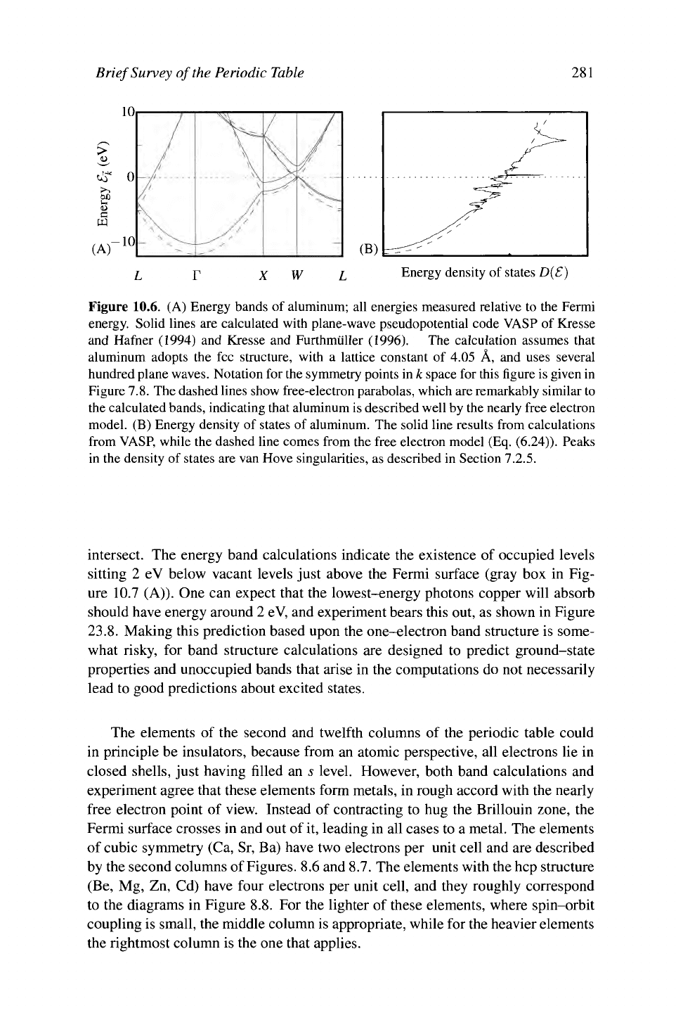
The band structure of aluminum appears in Figure 10.6. The calculated bands

are compared with free-electron parabolas, whose complicated appearance is purely

due to their reduction to the first Brillouin zone. The electrons in aluminum are be-

having nearly as if they were noninteracting electrons moving through an empty

box.

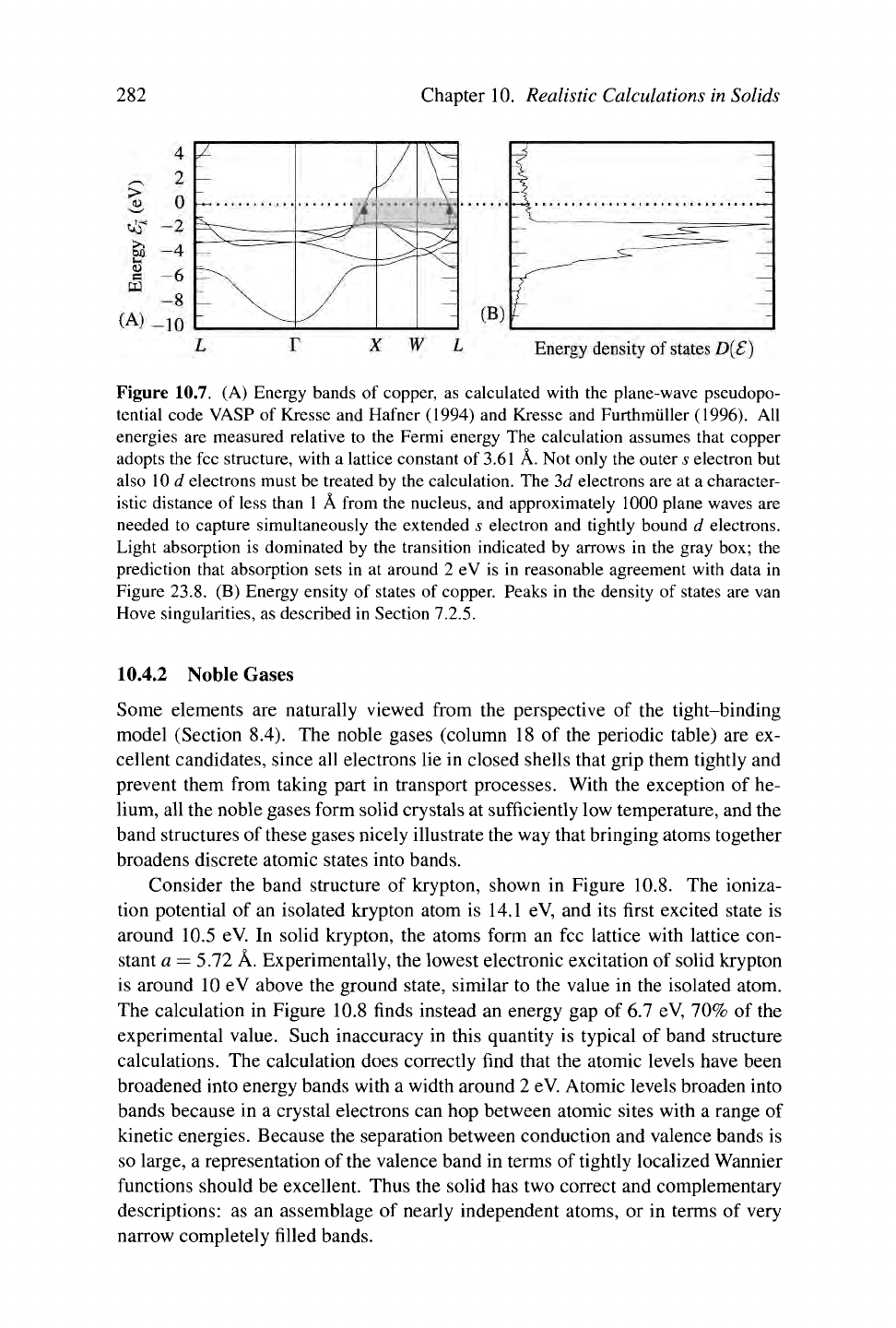
By contrast, the bands of copper shown in Figure 10.7 contain features both

of localized and nearly free electrons. The ten 3d electrons lie in a set of narrow

bands about 2 eV below the Fermi surface and about 2 eV in width, while the 4s

electron lies mainly in a band extending from about 10 eV below the Fermi surface

to several electron volts above. The density of states looks like the sum of two

pieces, the broad band containing the s electron, and the narrow band containing

d electrons. The s and d bands hybridize together in the energy range where they

Brief Survey of the Periodic Table

<ύ~

ËP

£ p X W L Energy density of states £)(£)

Figure 10.6. (A) Energy bands of aluminum; all energies measured relative to the Fermi

energy. Solid lines are calculated with plane-wave pseudopotential code VASP of Kresse

and Hafner (1994) and Kresse and Furthmuller (1996). The calculation assumes that

aluminum adopts the fee structure, with a lattice constant of 4.05 Â, and uses several

hundred plane waves. Notation for the symmetry points in k space for this figure is given in

Figure 7.8. The dashed lines show free-electron parabolas, which are remarkably similar to

the calculated bands, indicating that aluminum is described well by the nearly free electron

model. (B) Energy density of states of aluminum. The solid line results from calculations

from VASP, while the dashed line comes from the free electron model (Eq. (6.24)). Peaks

in the density of states are van Hove singularities, as described in Section 7.2.5.

intersect. The energy band calculations indicate the existence of occupied levels

sitting 2 eV below vacant levels just above the Fermi surface (gray box in Fig-

ure 10.7 (A)). One can expect that the lowest-energy photons copper will absorb

should have energy around 2 eV, and experiment bears this out, as shown in Figure

23.8.

Making this prediction based upon the one-electron band structure is some-

what risky, for band structure calculations are designed to predict ground-state

properties and unoccupied bands that arise in the computations do not necessarily

lead to good predictions about excited states.

The elements of the second and twelfth columns of the periodic table could

in principle be insulators, because from an atomic perspective, all electrons lie in

closed shells, just having filled an s level. However, both band calculations and

experiment agree that these elements form metals, in rough accord with the nearly

free electron point of view. Instead of contracting to hug the Brillouin zone, the

Fermi surface crosses in and out of it, leading in all cases to a metal. The elements

of cubic symmetry (Ca, Sr, Ba) have two electrons per unit cell and are described

by the second columns of Figures. 8.6 and 8.7. The elements with the hep structure

(Be,

Mg, Zn, Cd) have four electrons per unit cell, and they roughly correspond

to the diagrams in Figure 8.8. For the lighter of these elements, where spin-orbit

coupling is small, the middle column is appropriate, while for the heavier elements

the rightmost column is the one that applies.

281

282

Chapter 10. Realistic Calculations in Solids

Figure 10.7. (A) Energy bands of copper, as calculated with the plane-wave pseudopo-

tential code VASP of Kresse and Hafner (1994) and Kresse and Furthmiiller (1996). All

energies are measured relative to the Fermi energy The calculation assumes that copper

adopts the fee structure, with a lattice constant of 3.61 Â. Not only the outer s electron but

also 10

electrons must be treated by the calculation. The 3d electrons are at a character-

istic distance of less than 1 Â from the nucleus, and approximately 1000 plane waves are

needed to capture simultaneously the extended s electron and tightly bound d electrons.

Light absorption is dominated by the transition indicated by arrows in the gray box; the

prediction that absorption sets in at around 2 eV is in reasonable agreement with data in

Figure 23.8. (B) Energy ensity of states of copper. Peaks in the density of states are van

Hove singularities, as described in Section 7.2.5.

10.4.2 Noble Gases

Some elements are naturally viewed from the perspective of the tight-binding

model (Section 8.4). The noble gases (column 18 of the periodic table) are ex-

cellent candidates, since all electrons lie in closed shells that grip them tightly and

prevent them from taking part in transport processes. With the exception of he-

lium, all the noble gases form solid crystals at sufficiently low temperature, and the

band structures of these gases nicely illustrate the way that bringing atoms together

broadens discrete atomic states into bands.

Consider the band structure of krypton, shown in Figure 10.8. The ioniza-

tion potential of an isolated krypton atom is 14.1 eV, and its first excited state is

around 10.5 eV. In solid krypton, the atoms form an fee lattice with lattice con-

stant a = 5.72 Â. Experimentally, the lowest electronic excitation of solid krypton

is around 10 eV above the ground state, similar to the value in the isolated atom.

The calculation in Figure 10.8 finds instead an energy gap of 6.7 eV, 70% of the

experimental value. Such inaccuracy in this quantity is typical of band structure

calculations. The calculation does correctly find that the atomic levels have been

broadened into energy bands with a width around 2 eV. Atomic levels broaden into

bands because in a crystal electrons can hop between atomic sites with a range of

kinetic energies. Because the separation between conduction and valence bands is

so large, a representation of the valence band in terms of tightly localized Wannier

functions should be excellent. Thus the solid has two correct and complementary

descriptions: as an assemblage of nearly independent atoms, or in terms of very

narrow completely filled bands.