Marder M.P. Condensed Matter Physics

Подождите немного. Документ загружается.

15.

Fluid Mechanics

15.1 Introduction

Raise the temperature

almost any solid sufficiently, and

melts, passing into

liquid state. The transition

dramatic because

the change

mechanical prop-

erties.

From

structural point

view, the change

the solid

the the transition

point

the loss

long-range order, but there

normally no need

set up

neu-

tron scattering experiment

order

detect melting. Liquids flow

and

solids

not.

15.2 Newtonian Fluids

15.2.1 Euler's Equation

hydrodynamic description

of a

fluid,

one

specifies

velocity vector

every

point

space. To obtain

equation

motion,

it is

easiest

begin

adopting

a reference frame moving with

small volume

dV of

fluid.

If fdV is

the net force

acting upon this section

fluid,

and p its

mass density, then

the

acceleration

the small volume will be given by

f/p.

Now move back to the stationary reference

frame.

the velocity

the fluid

described by

v(r, t) at

time

then

short time

dt later

will

described by

v(r + vdt,t+dt)=v(r,t)+f(7,t)dt/p The

fluid

now at r

vdt was at? (15.1)

a time

ago.

=φ.

fy . VÌV = —.

Expand

first ordering/. (15.2)

The pressure

in a

fluid

defined

as the

force

per

unit area across

any

face

one

imagines inscribing within

it.

Therefore, the force

acting

on a

small volume

fluid may

identified with —VP, the gradient

the pressure, and Eq. (15.2)

can

be rewritten

Euler's equation

- VP

(v-V)v +

— =

0. (15.3)

The density

p of

a fluid does not have to be constant, but

must obey the equation

of continuity

——

—V ·

OU. This general statement of conservation of

mass

(15.4)

Qt first appeared

Eq. (5.25).

413

Condensed Matter

Physics,

Second Edition

by Michael P. Marder

414 Chapter 15. Fluid Mechanics

Equation (15.3) can be rewritten in the form of a continuity equation for the con-

servation of momentum, so that the time rate of change of momentum equals the

divergence of a momentum flux. The manipulations are simplest if one moves to a

component notation, rewriting Eq. (15.3) as

dpv

dp v^ 9 d „

,.,..+.

dt dt ^

Ci OD (1 Ci Ci

E^(m+V(·

(15.7)

Momentum in a small region changes because of two additive contributions: One

is from forces applied to the region, and the other is from fluxes of neighboring

fluid into the region. The fluid stress tensor σ is defined by

β = -ρν

αβ

Ρ,

(15.8)

leading Euler's equation to take the form

dpVr, v-^ d

-JL-^L = )T

—-σ

α0

Compare with Eq. (12.35). (15.9)

dt ^ dr

Incompressible Fluids. In many liquids, such as water, the change of pressure

needed to produce any appreciable change in density is larger than readily occurs

even in turbulent flows. In this case, the fluid is best approximated as incompress-

ible, the equation of continuity Eq. (15.4) becomes

V-w = 0, (15.10)

and the pressure P must be determined by the condition that the velocity v contin-

ually obey Eq. (15.10) while evolving according to Eq. (15.7).

The stress tensor in Eq. (15.8) has two physical interpretations. On the one

hand, Eq. (15.9) is in the form of a continuity equation, although missing a minus

sign that might be expected on the right-hand side, so σ

β gives the flux of mo-

mentum p

in the direction — r

. Sometimes the tensor n

g = — σ

β is defined so

as to alter this minus sign convention. The motivation for the sign convention of

Eq. (15.9) is to make it identical to the equation of linear elasticity in Eq. (12.35),

and corresponding to the sketch in Figure 12.3. Thus σ

β can also be interpreted

as the force along a per area exerted by material outside upon a fluid region of

interest.

Apart from the superfluids described in Section 15.5, no real liquid comes ter-

ribly close to obeying Euler's equation Eq. (15.7). A fluid obeying Euler's equation

conserves energy in the flow, and a swirl of liquid once started never decays. Real

fluids have dissipation and behave quite differently. The mathematical properties of

Newtonian Fluids

415

Euler's equation are uncertain. Despite tremendous effort, it is not known whether

nonsingular initial conditions remain nonsingular for all times, or whether flow can

concentrate into vortices whose rotation rate becomes infinite at some time, after

which the equations break down.

15.2.2 Navier-Stokes Equation

The correction of Euler's equation to allow for dissipation can take place in two

ways.

It can be done by considering the statistical mechanics of fluids and gases,

or through phenomenological arguments. In either event, the process is greatly

aided by having some idea of the form the theory should take.

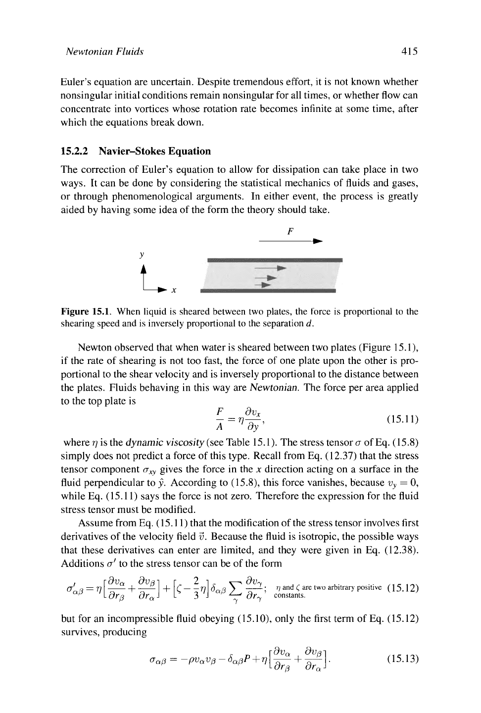
Figure 15.1. When liquid is sheared between two plates, the force is proportional to the

shearing speed and is inversely proportional to the separation d.

Newton observed that when water is sheared between two plates (Figure 15.1),

if the rate of shearing is not too fast, the force of one plate upon the other is pro-

portional to the shear velocity and is inversely proportional to the distance between

the plates. Fluids behaving in this way are Newtonian. The force per area applied

to the top plate is

where η is the dynamic viscosity

(see

Table 15.1). The stress tensor σ of

Eq.

(15.8)

simply does not predict a force of this type. Recall from Eq. (12.37) that the stress

tensor component σ^ gives the force in the x direction acting on a surface in the

fluid perpendicular to y. According to (15.8), this force vanishes, because v

= 0,

while Eq. (15.11) says the force is not zero. Therefore the expression for the fluid

stress tensor must be modified.

Assume from Eq. (15.11) that the modification of the stress tensor involves first

derivatives of the velocity field v. Because the fluid is isotropie, the possible ways

that these derivatives can enter are limited, and they were given in Eq. (12.38).

Additions σ' to the stress tensor can be of the form

'αβ = ν

9υ

dv-,

C 77 δ

β } -;

and

are two arbitrary positive (15.12)

1 -<-—' Qf ' constants.

'Ί

but for an incompressible fluid obeying (15.10), only the first term of Eq. (15.12)

survives, producing

β = -ρν

υβ-ο

βΡ + ηγ—

+ —

γ (15.13)

416

Chapter 15. Fluid Mechanics

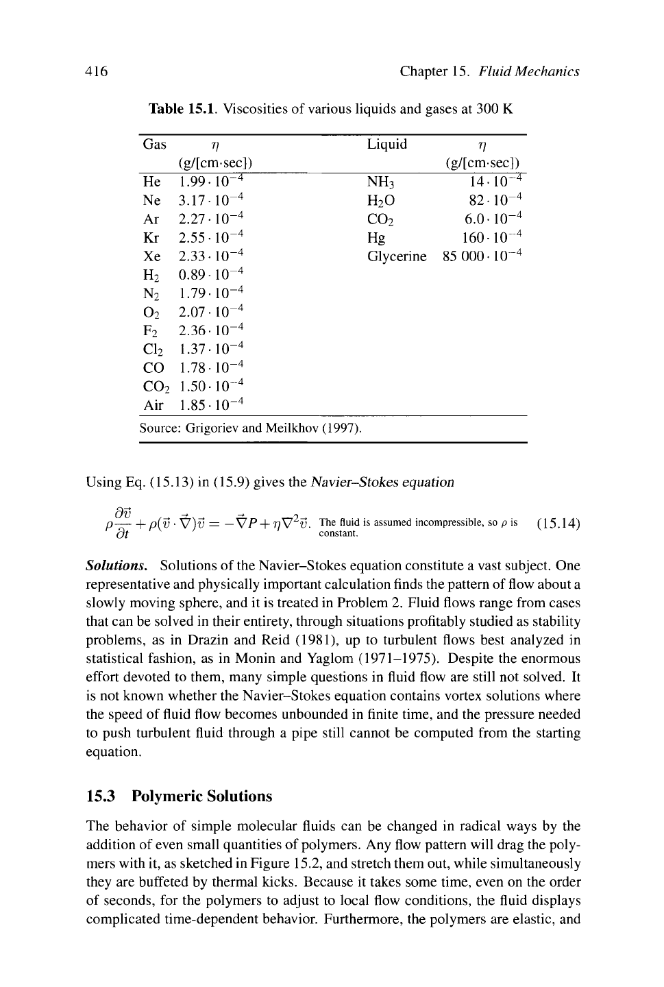
Table 15.1. Viscosities of various liquids and gases at 300 K

Gas

(g/[cm-sec])

1.99 ·10~

3.17

2.27

2.55

2.33

io-

IO"

Liquid

Glycerine

(g/[cmsec])

14·10~

82·IO"

6.0· IO"

160-IO"

85 000·IO'

-4

Source: Grigoriev and Meilkhov (1997).

Using Eq. (15.13) in (15.9) gives the Navier-Stokes equation

n \- p(v · Vìu =

—

VP + 77V V. The fluid is assumed incompressible, so p is (15.14)

dt constant.

Solutions. Solutions of the Navier-Stokes equation constitute a vast subject. One

representative and physically important calculation finds the pattern of flow about a

slowly moving sphere, and it is treated in Problem 2. Fluid flows range from cases

that can be solved in their entirety, through situations profitably studied as stability

problems, as in Drazin and Reid (1981), up to turbulent flows best analyzed in

statistical fashion, as in Monin and Yaglom (1971-1975). Despite the enormous

effort devoted to them, many simple questions in fluid flow are still not solved. It

is not known whether the Navier-Stokes equation contains vortex solutions where

the speed of fluid flow becomes unbounded in finite time, and the pressure needed

to push turbulent fluid through a pipe still cannot be computed from the starting

equation.

15.3 Polymeric Solutions

The behavior of simple molecular fluids can be changed in radical ways by the

addition of even small quantities of

polymers.

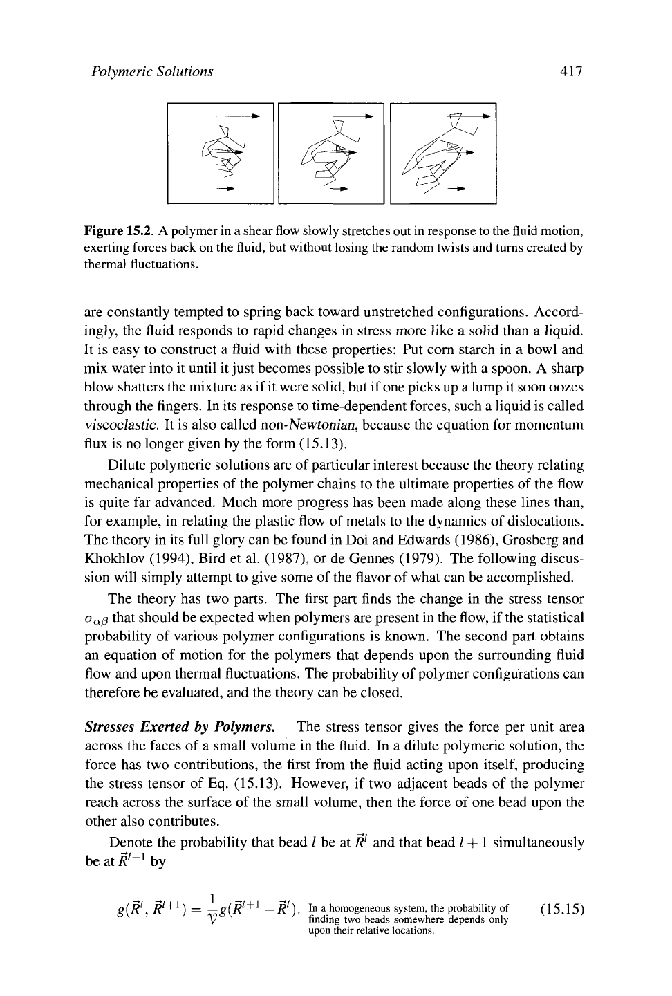
Any flow pattern will drag the poly-

mers with it, as sketched in Figure 15.2, and stretch them out, while simultaneously

they are buffeted by thermal kicks. Because it takes some time, even on the order

of seconds, for the polymers to adjust to local flow conditions, the fluid displays

complicated time-dependent behavior. Furthermore, the polymers are elastic, and

Polymeric Solutions All

Figure 15.2.

polymer

a shear

flow

slowly stretches out

response to the

fluid

motion,

exerting forces back on the

fluid,

but without losing the random twists and turns created by

thermal fluctuations.

are constantly tempted to spring back toward unstretched configurations. Accord-

ingly, the fluid responds to rapid changes in stress more like a solid than a liquid.

It is easy to construct a fluid with these properties: Put corn starch in a bowl and

mix water into it until it just becomes possible to stir slowly with a spoon. A sharp

blow shatters the mixture as if it were solid, but if

one

picks up a lump it soon oozes

through the fingers. In its response to time-dependent forces, such a liquid is called

viscoelastic. It is also called non-Newtonian, because the equation for momentum

flux is no longer given by the form (15.13).

Dilute polymeric solutions are of particular interest because the theory relating

mechanical properties of the polymer chains to the ultimate properties of the flow

is quite far advanced. Much more progress has been made along these lines than,

for example, in relating the plastic flow of metals to the dynamics of dislocations.

The theory in its full glory can be found in Doi and Edwards (1986), Grosberg and

Khokhlov (1994), Bird et al. (1987), or de Gennes (1979). The following discus-

sion will simply attempt to give some of the flavor of what can be accomplished.

The theory has two parts. The first part finds the change in the stress tensor

β that should be expected when polymers are present in the flow, if the statistical

probability of various polymer configurations is known. The second part obtains

an equation of motion for the polymers that depends upon the surrounding fluid

flow and upon thermal fluctuations. The probability of polymer configurations can

therefore be evaluated, and the theory can be closed.

Stresses Exerted by Polymers. The stress tensor gives the force per unit area

across the faces of a small volume in the fluid. In a dilute polymeric solution, the

force has two contributions, the first from the fluid acting upon

itself,

producing

the stress tensor of Eq. (15.13). However, if two adjacent beads of the polymer

reach across the surface of the small volume, then the force of one bead upon the

other also contributes.

Denote the probability that bead / be at R

and that bead / +

simultaneously

beatfl

/+1

Q(R

/?'+) = —g(R —R). In a homogeneous system, the probability of (15.15)

V finding two beads somewhere depends only

upon their relative locations.

418 Chapter 15. Fluid Mechanics

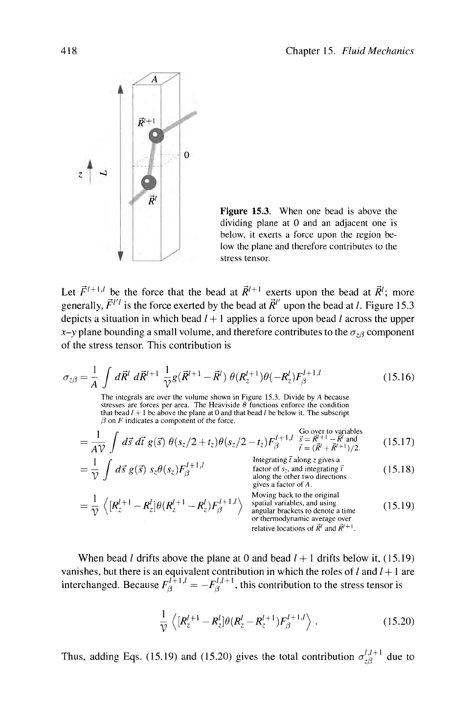
Figure 15.3. When one bead is above the

dividing plane at 0 and an adjacent one is

below, it exerts a force upon the region be-

low the plane and therefore contributes to the

stress tensor.

Let

l+l

be the force that the bead at

l+i

exerts upon the bead at R

; more

generally, F

' is the force exerted by the bead at R

upon the bead at /. Figure 15.3

depicts a situation in which bead / +

applies a force upon bead / across the upper

x-y

plane bounding a small volume, and therefore contributes to the σ

β component

of the stress tensor. This contribution is

°zß = \j dR

t+i

^g(R

l+i

-R

) 9(R

)9(-R{)F>+

(15.16)

The integrals are over the volume shown in Figure 15.3. Divide by A because

stresses are forces per area. The Heaviside

functions enforce the condition

that bead / +

be above the plane at 0 and that bead / be below it. The subscript

ß on F indicates a component of the force.

i r- Go over to variables

=— I dsdt

(s) e(s

/2+t

)e(s

/2-t

*:§:;>?,$

os.n)

\ f Integrating /along z gives a

= — / ds g(s) S

9(s

)Fß' factor of s

, and integrating T (15.18)

V J along the other two directions

gives a factor of A.

i Moving back to the original

= « < \

' - Ml

(R[

' - R[

)

' '' )

atial

variables, and using (15.19)

z zi \ z z) p I angular brackets to denote a time

or thermodynamic average over

relative locations of

Ä'

and

/?'

When bead / drifts above the plane at 0 and bead / +

drifts below it, (15.19)

vanishes, but there is an equivalent contribution in which the roles of / and / +

are

interchanged. Because Fß

' =

—F~

, this contribution to the stress tensor is

1 ([M+

-R

]e{R

-R[

) . (15.20)

Thus,

adding Eqs. (15.19) and (15.20) gives the total contribution σ '

due to

Polymeric Solutions

419

beads / and / + 1, which equals

... \ i /-LI ;\ The reason for the factor Ä

—R[ is that the

ζβ

V V-^

~^z*^ß ') larger the distance between «^+' and «J in (15.21)

* Figure

15.3,

the larger the probability that the

plane at 0 will lie between them.

1 <

i+i

i+hi\

i,M\

(l522)

- v V

I V \

z β

= τζ

(\RÌ

+Ì

)

+ -

(RÌ^FÌT

)

. Changing the labeling cannot (15.23)

P /V\

Z β

I affect the results.

The contribution to the stress tensor obtained by summing over all the beads is

«/3

= ^Σ(<^'

)·

(15

24)

//'

The subscript z has been replaced by a, because it does not matter whether x, y,

or z was chosen. This expression gives the contribution from the polymer beads,

and it must be added to the contribution from the fluid. Equation (15.24) follows

from Eq. (15.23) when beads interact with nearest neighbors, but it is true more

generally.

Polymer Equation of Motion. In order to evaluate Eq. (15.24) one needs to know

the probability that adjacent beads will differ in height by certain amounts, and then

to take averages. These probabilities depend upon the flow in which the polymer

finds

itself,

and also upon the magnitude of thermal fluctuations.

There are two common schemes to calculate the motions of polymers. The

first is called the Rouse model, and it treats the interaction between liquid and

polymer in a fairly naive way. In addition to a shearing force created by the fluid,

the polymer beads are subject to random kicks, and they interact with their nearest

neighbors. This calculation is oversimplified because of the way it treats the fluid

flow around the polymer. In reality, whenever a thermal fluctuation kicks one bead,

its motion moves the surrounding fluid and makes other beads move as well. Incor-

porating the rather long-range effective force between beads due to this effect leads

to the Zimm model. The word "model" is somewhat misleading because the effec-

tive interaction between beads mediated by the fluid is certainly real, and the only

question is whether the approximations used by Zimm (1956) are adequate to treat

the actual complexity. However, for the sake of simplicity, only the calculation of

Rouse (1953) will be presented here.

The motion of bead / is given by

= — ^2 F

— b(R

— v) + ξ

■

As before,

'>'

gives the force on bead / due (15.25)

Wl ,i to bead /'. m is the mass of the bead.

The form of this equation is in accord with the fluctuation-dissipation theorem

mentioned in Eq. (5.41). The constant b describes damping of the bead propor-

tional to the difference between its velocity and the local velocity of the fluid v.

420

Chapter 15. Fluid Mechanics

The random force ξ

is chosen so that while the time (or thermodynamic) average

of any component \ξ

) vanishes, the product of two components obeys

?/)A k ΤΛ(7ί Treating this time correlation function as a

(0)£a(t)\

{ I delta function means that the thermal kicks Q5 26)

xsav /SpV 11 ■ are very rapid in comparison with any other ^ ' '

dynamical process in the system.

How exactly one should think about the fluid velocity v is a matter that at first

seems simple, but then becomes complicated after further consideration. In the

view of Rouse (1953), v is simply the average fluid velocity in the vicinity of

the bead at R

, and the drag force on the bead is naturally the Stokes drag b =

βπηΐί found in Problem 2. The problem that Zimm (1956) noted with this point of

view is that the bead is not a single isolated sphere moving in a flow that arrives

asymptotically at a value of v. Other beads are nearby, interacting with the flow,

pushing at the bead in question whenever they move, and making it difficult to

determine how v is supposed to be measured.

Neglecting this difficulty, consider the case where particles have sufficiently

light mass and sit in a sufficiently viscous and slowly moving fluid that acceleration

of particles is negligible. Taking forces between nearest neighbors only, with spring

constant % as given by Eq. (5.67), Eq. (15.25) becomes

_; JC -, - -> ?

= v-\ [R

l+l

— 2R

+R'~

}

+ —. Eq. (5.67) calculated the spring constant X/N (15.27)

bin b ofyv monomers in series, while what is needed

here is the spring constant 3C between two

monomers.

Sticking with the simple view in which one pretends that the flow v can be set equal

to a large smooth macroscopic flow that might be observed externally, note that the

flow will vary with the precise location of the bead, but that for small motions and

slowly varying flows, only linear spatial variations of v should matter. Let W be

the tensor giving these variations:

Assume that the polymer is sufficiently small

„. _ r»0 , \

iy nl that W can be considered constant over its full nc 98')

a a

' j

P ß

extent. Different polymers at different loca- ^ ' '

tions may see different flow features, but each

one sees only a uniform shear flow.

Then Eq. (15.27) becomes

Ri =

U°

—\R

I+1

-2R

+R'-

} + -. (15.29)

bin b

The resemblance with the tight-binding model of Section 8.4 should suggest

the value of moving to Fourier components to solve Eq.

(

15.29).

Denote the Fourier

modes by

"φ = —■= y e [R —V t\. Subtracting v°t means going to a reference (15.30)

y N 7~f frame that moves with the mean flow, and N

is the total number of beads in the polymer.

Polymeric Solutions 421

Substituting Eq. (15.30) into Eq. (15.29) and neglecting the term Wv°t, which

vanishes for pure shear flows, and in any event is quadratic in velocities, gives

ψ<

= {W

)

ψ'+η-

ξ" = l/y/N

Σ ?

εχρ[2π/«//ν], (15.31)

With this normalization, ξ*

continues to obey Eq. (15.26).

with

= —

(l-cos[27rk/N\). (15.32)

If W is independent of

time,

one can write

lk_

[' JJ

„-U'-tW-Ui]^')

= dt e^

K >[

^-^—

. Remember that W is a matrix. (15.33)

In general W depends upon time, as the flow changes, and the polymer is swept

into new regions. In this case, it is easiest to solve Eq. (15.31) with perturbation

theory, first taking W

0 and then modifying the solution to first order in W.

this perturbative scheme,

dt'

^'~'^

Just set ^=0 in Eq. (15.33). The superscript (15.34)

0 means zeroth order in perturbation theory.

=►

{t)r

]

V))

^<W

(15.35)

This result will be useful shortly. It results from a brief calculation

employing Eq. (15.26) that is the subject of Problem 5.

^a-V^+Z

dt' Σ

Wß(t')ip

{t') Keep everything to order W. (15.36)

J-oo

J—oo

<*'

Σ «"«»'««.«'«"(O)

■

-iVSi«, <

1537

[δ

αβ

J^dt'

e-(

'^[W

ßa

(t')+W

aß

(t')]} .

(15.38)

Assembling the Pieces. In Eq. (15.24) the stress tensor is related to an average

over bead locations, while Eq. (15.38) evaluates an average of some Fourier trans-

forms of the locations. With a bit of extra manipulation, Eq. (15.38) turns out to be

just what is needed to find the stress tensor

σ.

Rewrite Eq. (15.24) as

°°β

ΐΣ,

W**)

Σ («

-24+^-

))

(15.39)

//'

— ^ (2 - 2

COS 2nk/N) (tpqlpff*) Invert Eq. (15.30) and replace/^ (15.40)

1 with V's; see Problem 5.

422

Chapter 15. Fluid Mechanics

mo y-^

k=\

Ψίψ"β

(15.41)

See Eq. (15.32). Why was the term k = 0 eliminated? Because ω^ = 0 for k = 0.

One might worry about factors of ω^ arising from Eq. (15.38). However, one can

see from Eq. (15.33) that perturbation theory gets the wrong answer when uj

= 0,

that ψ* is actually finite, and eliminating k = 0 from the present sum is correct.

k=l

δαβ

aß

ßo

Use Eq. (15.38) with W assumed constant in

time.

N/2

Νδ

αβ

2Σ

k=\

aß

+ w

ß0

Νδ

αβ

+ 2

k=\

aß

ßa

2XÌ_

/2nk\

~mb2 \N~)

Use (15.32), expand out the

cosine to leading order for

i<i/,

and extend the upper

limit of the sum to infinity,

because it converges.

Nö

aß

+ {W

aß

+ W

ßa

mbN

' \2%

The sum ^

■-n

(15.42)

(15.43)

(15.44)

(15.45)

was performed in Problem 6,

Eq. (6.83) in Chapter 6.

The first term of Eq. (15.45) leads to a uniform decrease of fluid pressure; the

osmotic pressure tries to surround polymers with as much fluid as possible, and

will try to suck water away from regions with lower density of polymer to make it

happen. The second term corresponds to an increase in viscosity.

Uniform Viscosity. Suppose, for example, that the flow v is a uniform shear flow

where v

increases linearly in the y direction, so

Wxy

= dv

/dy is nonzero but all

other components of W vanish. Then

' xy

T N

ÜX^y-

(15.46)

Compare with Eq. (15.13) and assume that instead of one polymer, there is a con-

centration c/N of polymers per unit volume, where c is the number of monomers

per unit volume, and N is the number of monomers per polymer. Then the viscosity

of the fluid is enhanced by an amount

δη

c N

—k

Tmb——

N \2X

1„2

c , N

—

—mo

N 12

The increase in the viscosity η. (15.47)

See Eqs. (5.66) and (5.67), which express the

(15.48)

spring constant 3Cas

= kgT/a

Problem 6 determines the frequency dependence of the viscosity. If a shear

velocity field oscillates as

Wxy(t)

cos ut, then

N-l

k=\

ν(ω

[uJk

cos

ujt

sin

cot].

(15.49)