Marder M.P. Condensed Matter Physics
Подождите немного. Документ загружается.

16.
Dynamics of Bloch Electrons
16.1 Introduction
Condensed matter physics provides an enormously successful account of the elec-
trical properties of solids. The reason for this success is not so much because
agreement between theory and experiment is better in this area than in any other,
but because many surprising and productive qualitative concepts have emerged.
The central idea is that response of a solid to weak electric and magnetic fields is
determined by the energy band curves £^. First derivatives of these curves give
effective velocities of electrons, while second derivatives give effective masses.
When the second derivatives are negative, the solid can behave as if filled with
particles with positive charge, called holes. All these dynamical phenomena result
in fact from interactions between electrons and the lattice potential, but the simple
ideas are so powerful that it is possible to forget all the theoretical underpinnings
and adopt a few apparently classical dynamical rules. Much of modern electronics
is built on this foundation.
16.1.1 Drude Model
The electron was only a few years old when the first theories of electrical conduc-
tion of metals appeared, by Drude (1900), Thomson (1907), and Lorentz (1909).
The Drude model imagines that a metal contains a population of electrons that are
accelerated by external electrical and magnetic fields, and are damped by some sort
of frictional force. They obey
-> v -* v
mv =
—eE —
e- x B
—
m-, (16.1)
c T
where r is a coefficient describing the damping and is called the relaxation time.
It acquires this name because if an electron is given an initial velocity
VQ
and let
loose in a solid without either electrical or magnetic fields present, the electron's
subsequent behavior is
v(t) = Vn£~ •
T
g'
ves
the characteristic time for any fluctu- (16.2)
ation to decay.
In the presence of an electrical field E, an initial velocity vo develops instead to
v(t) =
E+[VQ-\
E}e~''
T
Assume a solution of the form A + Be~'/
T
(16.3)
tïl m and solve for the unknown constants.
453
Condensed Matter
Physics,
Second Edition
by Michael P. Marder
Copyright © 2010 John Wiley & Sons, Inc.
454 Chapter 16. Dynamics of Block Electrons
so that at times much longer than r one obtains
re -
E Equivalent to observing that at long times v
m win stop changing, so one can just set v to
zero in Eq. (16.1) and solve for v.
(16.4)
If the density of mobile electrons is n, then the current density j arising in response
to E is
(7 :
-nev
ne
2
r
m
ne
2
r
m
(16.5)
(16.6)
where the electrical conductivity a is defined to be the linear coefficient relating
current flow to electrical field.
Measurements of electrical conductivity are usually reported in terms of its
inverse, the resistivity p, in terms of which the relaxation time can be expressed as
m
ne
2
p
3.55-10
13
n/[\0
22
cm"
3
] p/[pÜ cm]
(16.7)
Using the resistivities from the periodic table inside the front cover in Eq. (16.7)
shows that the relaxation time is on the order of 10~
14
s. By
itself,
this calcula-
tion does not seem to make any real predictions, because it determines electrical
conductivity only at the expense of introducing another unknown, the relaxation
time.
It does, however, frame electrical conductivity in the terms that will be used
later for more detailed calculation, as a balance between the force — eE causing
electrons to accelerate, with the damping from scattering events encoded in r that
causes them to decelerate.
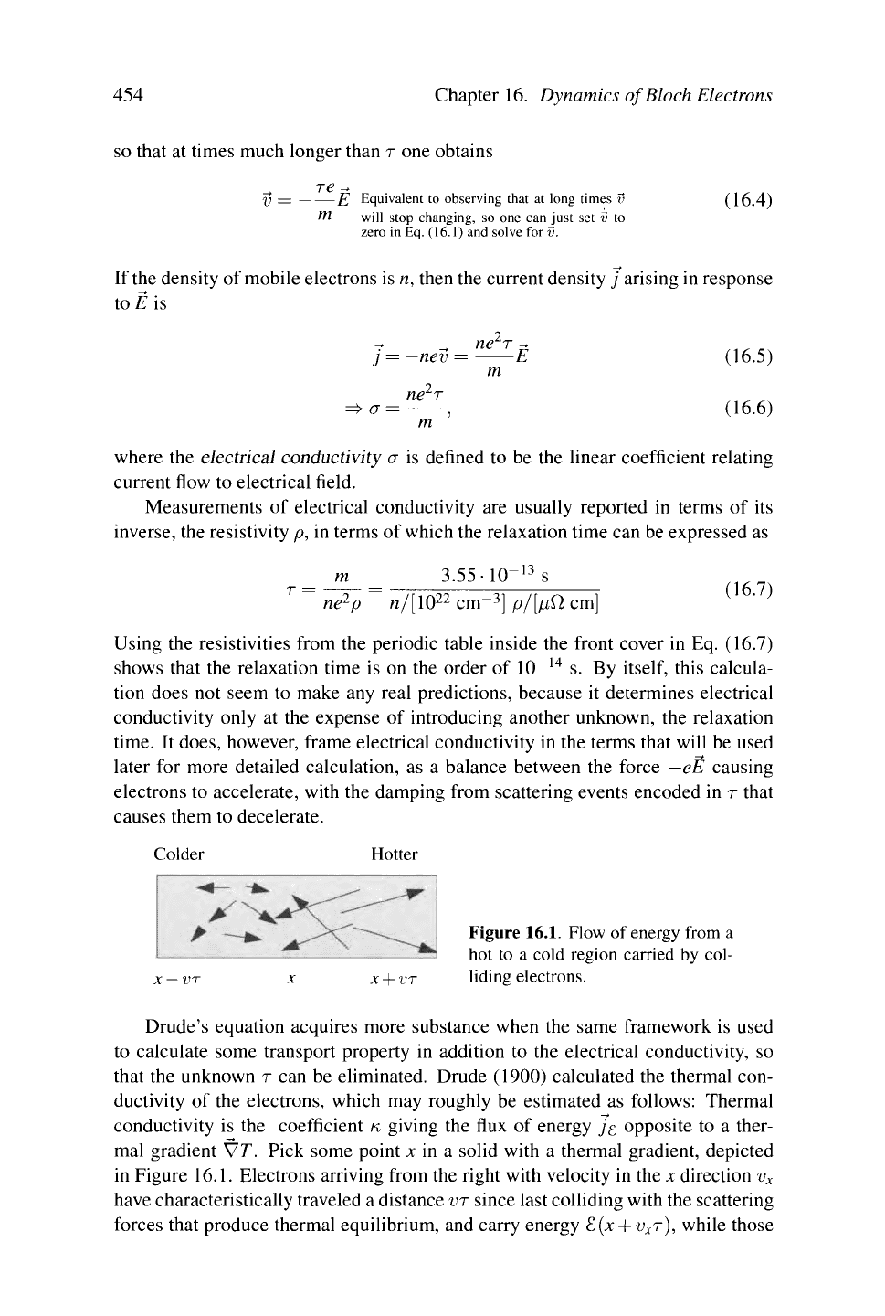
Colder Hotter
Figure 16.1. Flow of energy from a
hot to a cold region carried by col-
liding electrons.
Drude's equation acquires more substance when the same framework is used
to calculate some transport property in addition to the electrical conductivity, so
that the unknown r can be eliminated. Drude (1900) calculated the thermal con-
ductivity of the electrons, which may roughly be estimated as follows: Thermal
conductivity is the coefficient K giving the flux of energy _/g opposite to a ther-
mal gradient V7\ Pick some point x in a solid with a thermal gradient, depicted
in Figure 16.1. Electrons arriving from the right with velocity in thex direction v
x
have characteristically traveled a distance
VT
since last colliding with the scattering
forces that produce thermal equilibrium, and carry energy
8.(X
+
V
X
T),
while those
Semiclassical Electron Dynamics
455
coming from the left carry energy
£ (x —
V
X
T)
.
The density of electrons arriving
from the right is something like
n/2
because half the electrons to the right have
positive velocities. So the net flux of energy is roughly
JE
=
-jV
x
\£{X-V
X
T)-£(X
+
V
X
T)\ K.
~nv
A
x
T—
=
-
nv
x
T
^f^
c
(
16
-
8
)
In
1
2
dT
rn
3k
2
B
T
dT
—
-mv
x
cyT—-
= —- -
r
- ,--.
m
2 OX m 2 OX
classically equal to
3k
B
/2,
while
average
x kinetic energy is
k
B
T/2.
mvicyT—-
=
Specific heat is
d£/97\
(16.9)
O)
" "
.-.-...
^
^_
=
3 fkß\
= 1 24 10
-13
cm
-l
K
-2
(16 10)
<JT
2 \ e J
Through
what was arguably a logical error, Drude originally obtained twice this
value,
in rather good agreement with experiment.
The argument used here to obtain the thermal conductivity does not stand up at all
to close inspection.
It
pretends that electrons all traveling with mean velocity
v
x
carry differing amounts of kinetic energy. The most that can be said for it is that it
is dimensionally sound and makes an essentially correct prediction, which is that
the thermal conductivity divided by electrical conductivity and temperature yields
a constant for metals. This fact was observed by Wiedemann and Franz (1853),
and the experimental constant is around 2.3
•
10~
13
erg cm
-1
K
-2
.
Producing
a
theory substantially better than these crude estimates requires
a
fair amount of effort, and will occupy the next two chapters. The first point to ad-
dress is the fact that distinct energy bands, indexed by n, are dynamically separate.
Under influence of weak and slowly varying fields, an electron that begins in one
band can easily move about among energy states in the same band, but is exponen-
tially unlikely to move into another. Next, by constructing an effective Lagrangian
for wave packets,
it
will be shown how electrons can act like classical particles
despite being described by Bloch's theory as waves. Finally, Boltzmann's general
framework for describing electrical and thermal transport of classical particles will
be used to predict the thermoelectric properties of metals.
16.2 Semiclassical Electron Dynamics
Rules
of
Semiclassical Dynamics. For many purposes, electrons
in
periodic
solids act like classical particles with slightly unfamiliar laws of motion. Before
beginning the lengthy process of deriving, justifying, and analyzing these laws,
it
is best to begin simply by stating what they are.
1.
The band index n is a constant of the motion. An electron that begins its life
in one band remains in it thereafter. For this reason, the band index n can be
omitted from energies and wave functions in the following discussion.
2.
The position of an electron in
a
crystal with inversion symmetry evolves ac-
cording to
•
10£r
r=
=*.
(16.11)
ft
Ok
456
Chapter 16. Dynamics of Block Electrons
3.
The electron's wave vector obeys
A _ e
■
-
Hk
= —eE rxB
(16.12)
where È and B are electric field and magnetic induction and may be spa-
tially varying. Because all energy functions and wave functions are periodic
functions of k, k is physically indistinguishable from k + K, where K is any
reciprocal lattice vector.
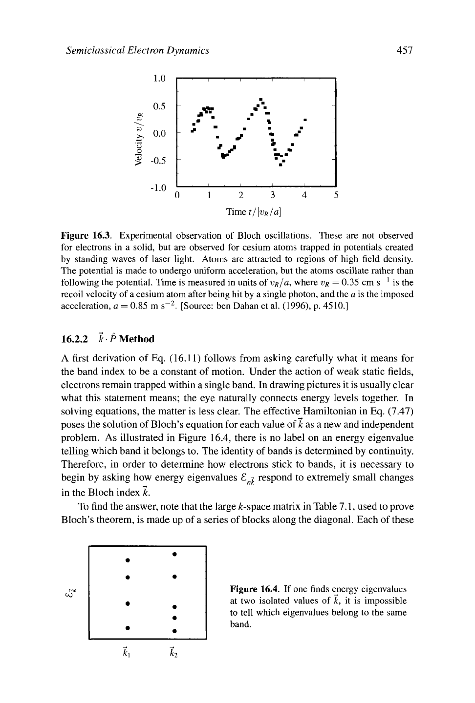
16.2.1 Bloch Oscillations
Although representing a semiclassical picture, many quantum-mechanical effects
are retained in Eqs. (16.11) and (16.12). These result from the fact that E^ is a
periodic function of k, as well as from the fact that the electron states are occupied
according to the Fermi distribution rather than according to classical statistical me-
chanics.
OJ
3ir/a
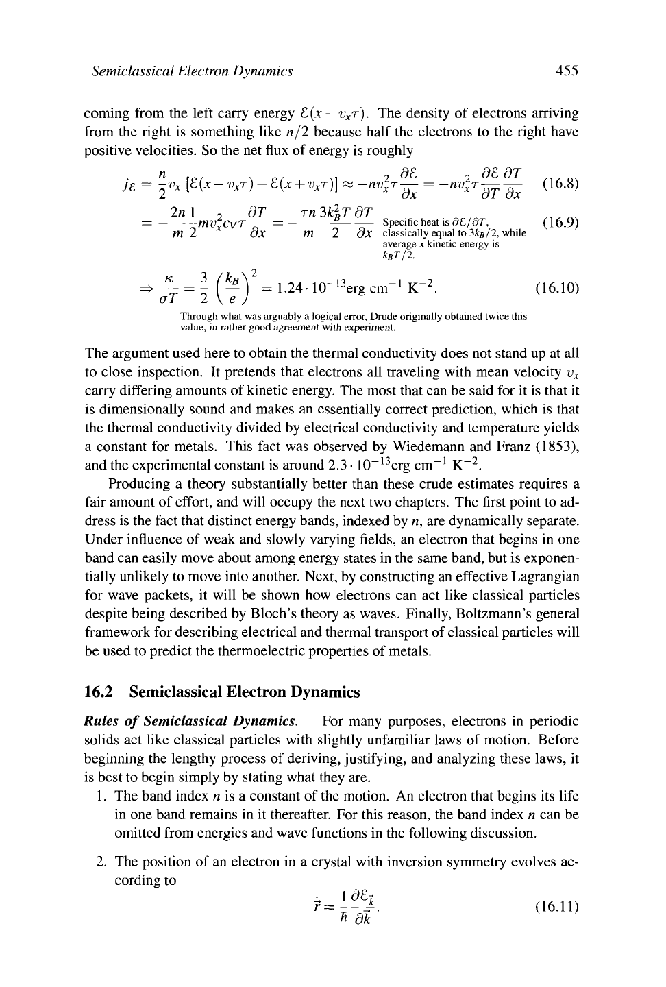
Figure 16.2. Energy of a tight- binding
band,
Eq.
(16.13). Electrons have negative
effective masses at k = ir/a and positive
effective masses at k = 0.
As an example, consider the semiclassical dynamics of electrons whose energy
is given by the tight-binding model, Eq. (8.72). For simplicity, specialize to a one-
dimensional lattice of lattice constant a and write the energy functional as
-2t cos ak, (16.13)
as shown in Figure 16.2. In the presence of a uniform electric field E, one has
From Eq. (16.12).
Hk
=
—eE
>k = -eEt/h
2 ta . /aeEt\
4>r= Sin From Eq. (16.11).
2t /aeEt\
cos
K-r)-
(16.14)
(16.15)
(16.16)
(16.17)
eE
V
H
The location of the electron oscillates in time; this behavior is called Bloch
oscillation. Despite the fact that k increases without bound, the mean position
of the electron is fixed. If this phenomenon were commonly seen, it would mean
that under sufficiently intense electric fields electrons would start to oscillate rather
than travel, and metals would become insulators. This simply does not happen. As
shown in Problem 2, small amounts of damping added to Eq. (16.14) destroy the
phenomenon, and electric fields in metals cannot practically be made large enough
to overcome it. However, under special circumstances, Bloch oscillation can be
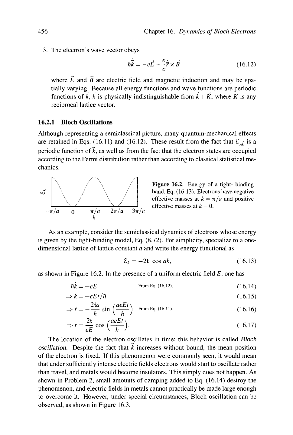
observed, as shown in Figure 16.3.
Se mie las sic al Electron Dynamics
457
£
1.0
0.5
0.0
-0.5
-1.0
2 3
Time f/[v«/a]
Figure 16.3. Experimental observation of Bloch oscillations. These are not observed
for electrons in a solid, but are observed for cesium atoms trapped in potentials created
by standing waves of laser light. Atoms are attracted to regions of high field density.
The potential is made to undergo uniform acceleration, but the atoms oscillate rather than
following the potential. Time is measured in units of
VR/Ü,
where
VR
= 0.35 cm s
_1
is the
recoil velocity of a cesium atom after being hit by a single photon, and the a is the imposed
acceleration, a = 0.85 m s~
2
. [Source: ben Dahan et al. (1996), p. 4510.]
16.2.2 k P Method
A first derivation of Eq. (16.11) follows from asking carefully what it means for
the band index to be a constant of motion. Under the action of weak static fields,
electrons remain trapped within a single band. In drawing pictures it is usually clear
what this statement means; the eye naturally connects energy levels together. In
solving equations, the matter is less clear. The effective Hamiltonian in Eq. (7.47)
poses the solution of Bloch's equation for each value of k as a new and independent
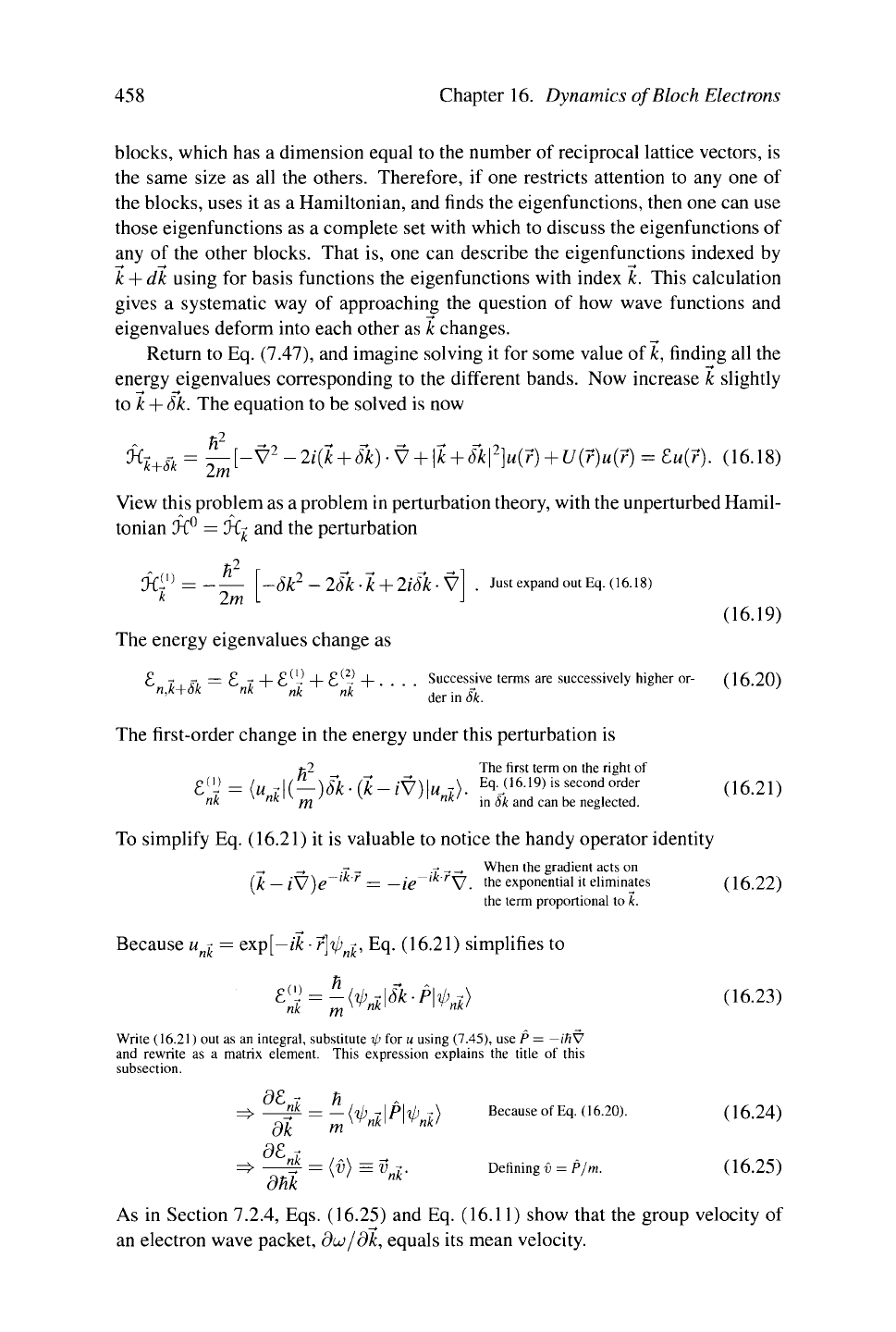
problem. As illustrated in Figure 16.4, there is no label on an energy eigenvalue
telling which band it belongs to. The identity of bands is determined by continuity.
Therefore, in order to determine how electrons stick to bands, it is necessary to
begin by asking how energy eigenvalues E
n
^ respond to extremely small changes
in the Bloch index k.
To find the answer, note that the large &-space matrix in Table
7.1,
used to prove
Bloch's theorem, is made up of a series of blocks along the diagonal. Each of these
Figure 16.4. If one finds energy eigenvalues
at two isolated values of k, it is impossible
to tell which eigenvalues belong to the same
band.
k\ k
2
458
Chapter 16. Dynamics of Block Electrons
blocks, which has a dimension equal to the number of reciprocal lattice vectors, is
the same size as all the others. Therefore, if one restricts attention to any one of
the blocks, uses it as a Hamiltonian, and finds the eigenfunctions, then one can use
those eigenfunctions as a complete set with which to discuss the eigenfunctions of
any of the other blocks. That is, one can describe the eigenfunctions indexed by
k + dk using for basis functions the eigenfunctions with index k. This calculation
gives a systematic way of approaching the question of how wave functions and
eigenvalues deform into each other as k changes.
Return to Eq. (7.47), and imagine solving it for some value of k, finding all the
energy eigenvalues corresponding to the different bands. Now increase k slightly
to k +
Ok.
The equation to be solved is now
H
2
- - - -
K
l+Sk
= —[-V
2
-2i{k + 8k)-V +
\k
+ 5k\
2
}u{r) + U(r)u{r) =
E,u(r).
(16.18)
View this problem as a problem in perturbation theory, with the unperturbed Hamil-
tonian Ä
0
=
'K-j,
and the perturbation
«-
"
2
-ök
2
-2ök-k + 2iök-V
k
2m
The energy eigenvalues change as
Just expand out Eq. (16.18
(16.19)
P - -. = P —L £'L -4- P^
2
} -4- Successive terms are successively higher or- (1620)
n,k+Sk nk nk nk j • F, '
* "* der in ok.
The first-order change in the energy under this perturbation is
»-2 The first term on the right of
P,°}
= (ui\( — )ök-(k-iV)\ur). Eq.J16.19) is second order (16.21)
nk
m
m in 6k and can be neglected.
To simplify Eq. (16.21) it is valuable to notice the handy operator identity
_, _ - .j _ _ When the gradient acts on
(£_
/V)e
r
= —/e
_
V. the exponential it eliminates (16.22)
the term proportional to k.
Because u
-^
=
exp[—ik-7]ip
n
^,
Eq. (16.21) simplifies to
h
J
nk ~
m^^nk
1
""'
'
]Y
nk
^l =
-Mnk\^-^nÙ
(16-23)
Write (16.21) out as an integral, substitute ip for u using (7.45), use P =
—iHV
and rewrite as a matrix element. This expression explains the title of this
subsection.
op
*-
=> —^ = -(lp
t\P\lp
t) Because of Eq. (16.20). (16.24)
dk m
nk
=^
™={V)=VT.
Defining v = P/m. (16.25)
dhk
n
As in Section 7.2.4, Eqs. (16.25) and Eq. (16.11) show that the group velocity of
an electron wave packet, du/dk, equals its mean velocity.
Noninter-acting
Electrons in an Electric Field 459
16.2.3 Effective Mass
External electric and magnetic fields accelerate electrons, forcing them to glide
along the energy bands. Suppose that these fields are very weak and that the change
in k is accordingly very slow. If it is sufficiently slow, then one can invoke station-
ary perturbation theory, as in the previous section, and argue that
dt
y
\ = \ —- -
— v
a
is the ath component oft). (16 26)
p
dk
ß
dt
(v)=hM-
l
k, (16.27)
where
1
9%ï
h
2
dk
a
dkß
(^~
l
)aß
=
-2^-^t-
FromE
i-
(16
'
25)
-
(16-28)
The tensor M defined in Eq. (16.28) is called the effective mass
tensor.
Because the
energy £^ is in general not isotropic, acceleration will not in general be parallel to
k. However, that is not the most interesting feature of the effective mass. Because
£ £ is a periodic function in k, its second derivatives will sometimes be positive
and sometimes negative. For example, in Figure 16.2, the inverse effective mass is
negative at k = ir/a and positive at k = 0. According to Eq. (16.12), the index k
always increases in the direction of decreasing electric fields. However, when the
effective mass is negative, the velocity of electrons is in the direction opposite to
k. Rather than thinking of these electrons as having negative mass, one thinks of
them as having positive charge and calls them holes.
Additional information on the effective mass tensor can be obtained by contin-
uing the perturbation expansion of Eq. (16.20) to second order. Problem 3 shows
that it can be written as
(M
-1
}
I,
+
1_
E
{^iPal^X^l^l^+CC.
n'^n
nk n'k
"c.c."
means "add the complex conjugate of the previous term." The sum is
carried out only over n!—not over n.
One can interpret Eq. (16.29) as saying that the effective mass of an electron arises
from virtual transitions between bands. The closer the energy E
n
,^ of band n' is to
the energy
£-
n
^
of band n, the larger the deviation of the inverse effective mass from
\/m will be. A nearby band of higher energy tends to make the effective mass
negative, while a nearby band of lower energy tends to make the effective mass
positive.
16.3 Noninteracting Electrons in an Electric Field
Understanding why electrons obey the semiclassical equations and why they are
not able to change band index requires considering the behavior of noninteracting
electrons placed in a weak electric field. This calculation is plagued with technical
460 Chapter 16. Dynamics of Block Electrons
difficulties. Periodic boundary conditions have played an important role in simpli-
fying the mathematics of the electrons, but it appears that when a uniform electric
field is turned on, one must abandon them. The electrostatic potential V(r) = — E
■
7
of a uniform electric field grows linearly in space, and so it must be larger at one
side of the sample than at the other. As a reflection of this fact, if one actually
places a finite sample of metal in an electric field, surface charges build up and
cancel out the field in the interior altogether.
There are two solutions to this difficulty. The method to be pursued in this
section recasts the problem so that the linear potential is eliminated altogether.
This technique allows great formal progress, including a calculation of the rate
of transitions between bands, but is hard to generalize so as to include magnetic
fields. The following section proceeds instead by restricting attention to a subset
of all wave functions, which are localized in space and therefore cannot see the
divergences in the electrical potential.
To recast the problem, eliminating the scalar potential V, note that one is inter-
ested in electric fields under conditions where electrons flow continually around in
a loop, and charge does not build up at the edges of the sample. A trick permit-
ting such a calculations follows from recalling that electric fields are generated by
time-dependent vector potentials according to Maxwell's equation
1 ÔA - Use ß = V x A in Eq. (20.5b), and
observe
E = W.
that
if the
curl
of
a function
vanishes,
it
equals
(16.30)
C dt the
gradient
of a
scalar.
By introducing a time-dependent vector potential A(t), one can generate an electric
field even when the scalar potential V vanishes. The advantage of employing A
rather than V is that it remains perfectly legitimate to work with periodic boundary
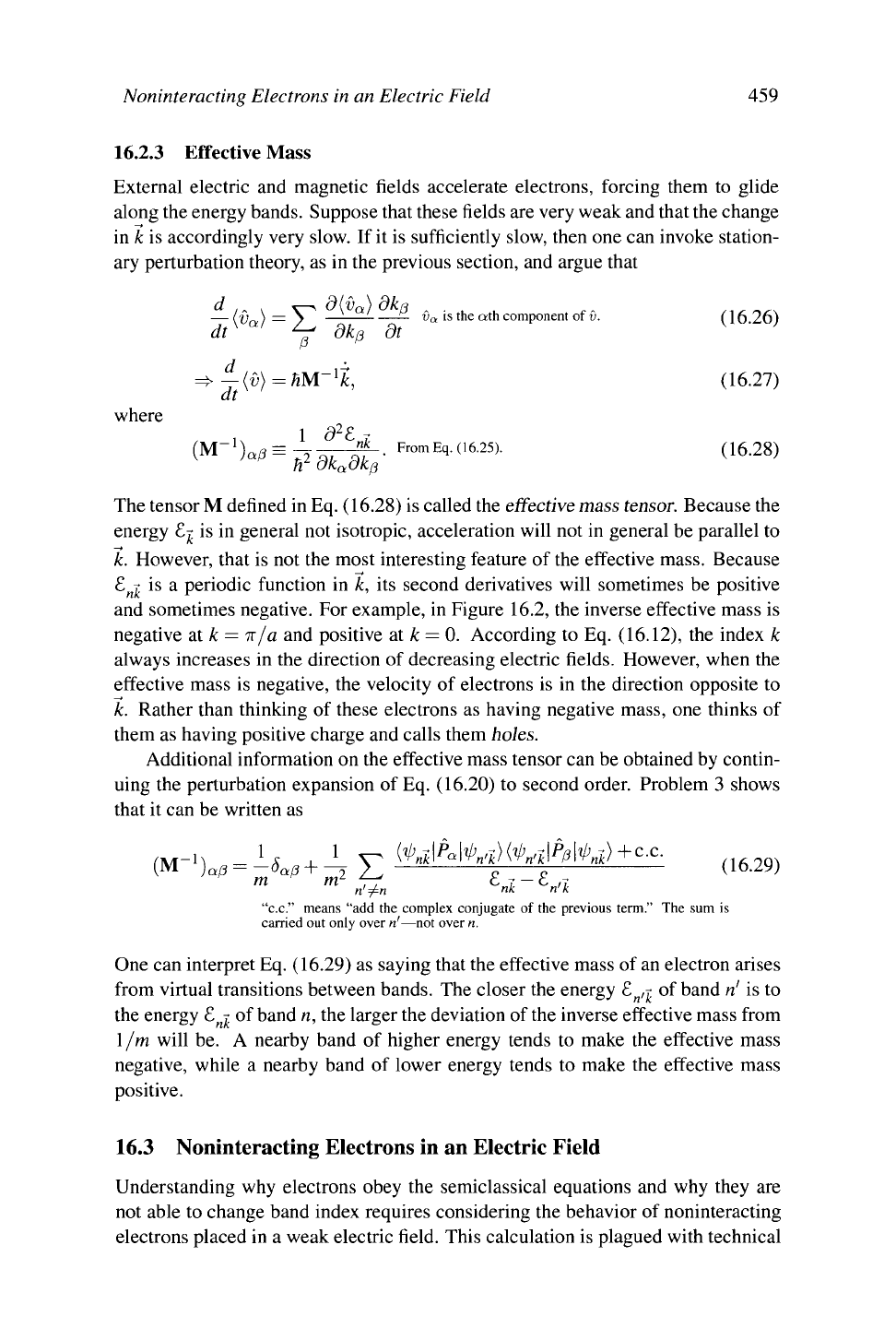
conditions. A convenient one-dimensional geometry is illustrated in Figure 16.5.
Mathematically, there is no difficulty at all in passing a thin tube of magnetic flux
through the middle of a loop of wire, although experimentally it is difficult to
achieve this feat without having some magnetic induction escape the thin tube and
impinge upon the wire.
Rather than focus upon details of a loop of wire, it is simplest to pose a one-
Figure 16.5. A thin tube of increasing mag-
netic flux through a loop of wire, so thin
that no magnetic induction is visible in the
wire,
generates a constant electromotive force
around the loop. The magnetic flux tube cor-
responds to a vector potential A parallel to
the wire and of strength —cEt, allowing an
electric field to coexist with periodic bound-
ary conditions. This geometry is the setting
for the definition of the Houston states.
Magnetic flux tube
B
z
= 2TT:R cEt 6(7)
Noninter-acting
Electrons in an Electric Field
461
dimensional problem, making use of
Eq.
(16.30). The Hamiltonian is
Û=^-(P+-A)
+Û(R),
(16.31)
2m \ c J
where
A = -cEt. (16.32)
Notice that the potential and hence the Hamiltonian are explicitly time-dependent.
This is the price one pays for the ability to impose periodic boundary conditions.
In order to solve (16.31), define
2m \ c
(x
t) = E[d)(x t). The subscript f on £ serves as a reminder that
£
is time-dependent.
(16.33)
The function
<f>(x,
t) is an eigenfunction of the Hamiltonian at any given time,
viewing time as a parameter. Because it resides on the loops shown in Figure 16.5,
it must be a periodic function and obey
d>(x-\-L)
=
<b(x).
Taking L to be the circumference of
the
loop.
(16.34)
Glancing back at Eq. (16.22) shows that by multiplying wave functions with a
phase factor, constants added to gradients can be induced to disappear. In fact, one
can eliminate the vector potential A from Eq. (16.33) altogether by defining
4>(x,
t) = e~
ieAx
'
hc
${x, t). (16.35)
Using Eq. (16.22) shows thatEq. (16.33) becomes
P
2
-
[— +
U]</>(x,t)
=
Z
t
<l>(x,t).
(16.36)
Equation (16.36) is nothing but Bloch's equation and its solutions are Bloch eigen-
states
4>nk(,){x)
=e
lk{
'
)x
U
n
i
iU
-
]
(x).
Where u
nk
is a periodic function, and k, like (16.37)
£, depends upon
time.
Disturbingly, the electric field appears to have vanished from the problem al-
together. Where did it go, and why are the energies and wave vectors shown de-
pending upon tl The answer is quite subtle. The electric field cannot really have
disappeared from the problem, and because the only part of
the
mathematical prob-
lem not dealt with carefully so far is the imposition of boundary conditions, that
is where the electric field must reside. Inserting Eqs. (16.35) and (16.37) into the
boundary condition (16.34) and recalling that u
n
^
t)
is periodic gives immediately
that
e
-ieA{x+L)/nc
e
ik(,){x+L)
Unk
^
x
+ L) = e
-ieAx/*c+ik(,)x ^
(16
_
3g)
462 Chapter 16. Dynamics of Bloch Electrons
-eA ,
nc
eEt ,
=>
-—+k(,)
n
2TTI
~~L'
2TT/
~~L'
Because
"nk(,)(
x
+
L
) =
u
nk(,)(
x
)-
/is
some
integer.
(16.39)
(16.40)
(16.41)
It follows from Eq. (16.40) that if the boundary conditions are to be obeyed, the
wave vectors k are indeed time-dependent, obeying
hk=-eE.
(16.42)
Despite the influence of the periodic potential U, the index k obeys classical
equations of motion for an electron in an electric field. The identical semiclassical
result is derived by another route in Problem 7.
The functions
4>
are
called Houston functions. The Houston functions are
orthonormal wave functions, but they are not exact solutions of Schrödinger's
equation, because as soon as eigenvalues are time-dependent, the connection be-
tween the time-dependent Schrödinger equation and an eigenvalue problem such
as Eq. (16.33) has been lost. If one starts an electron in a particular Houston state
at t = 0 and follows its time evolution, it begins to deviate from a perfect Houston
state in two ways. First, as it evolves, the amplitudes of Houston states with nearby
k become nonzero and grow, as shown in Problem 8. This behavior is typical of
wave packets, and it corresponds to the spread of the wave packet under the in-
fluence of Schrödinger's equation. The spread cannot be prevented, although its
effects can be minimized by starting the electron in a superposition of states with
nearby k. In addition to this gradual spread of wave vectors within a band, there is a
more interesting phenomenon where the electron jumps from one band to another,
a phenomenon known as Zener tunneling.
16.3.1 Zener Tunneling
Rough Calculation. One way to explain Zener tunneling is to observe that the
effect of an electric field is to change electrons' energy by eE
■
r, so that the band
energy £ ^ shifts up and down with position, as shown in Figure 16.6. Suppose that
an electron sits at the top of a valence band, E
v
, and the bottom of a conduction
band £
c
sits a distance £
g
above it. If the electron can jump over a distance
£
g
/eE,
then without changing energy, it can enter the conduction band. The problem is
that during this voyage, it will need to have an energy lying in the gap between
valence and conduction bands.
It is not precisely true to say that states with energies lying in the energy gap are
forbidden. They exist, but only if one permits complex values of the Bloch index
k. Because these solutions grow exponentially, they cannot uniformly fill a macro-
scopic crystal. According to the WKB approximation, introduced in Eq. (4.9), the
amplitude for an electron to tunnel from one band to another should roughly be of
the form