Marder M.P. Condensed Matter Physics
Подождите немного. Документ загружается.

Localization
543
only argue that adding two impurities creates two bound states, three impurities
three, and so on. One would conclude in this way that when an impurity is added
to every site in one dimension, all states are localized. In two dimensions, they
should also be localized, although the binding energies and decay lengths might be
exponentially small. In three dimensions, only if the disordering wells had a height
on the order of 9t might one expect all states to be localized, and one would have
to consider the possibility that some states might be localized, and others not.
All these conclusions are correct, although the arguments are very imprecise.
In fact, the conclusions can break down when one has added as few as two im-
purities to a system. Two impurities in a one-dimensional system do not neces-
sarily create two bound states. If they are close together, they may merge into a
single well, leaving still a single bound state. Nevertheless, for typical samples,
the consensus has it that the situation in one, two, and three dimensions stands as
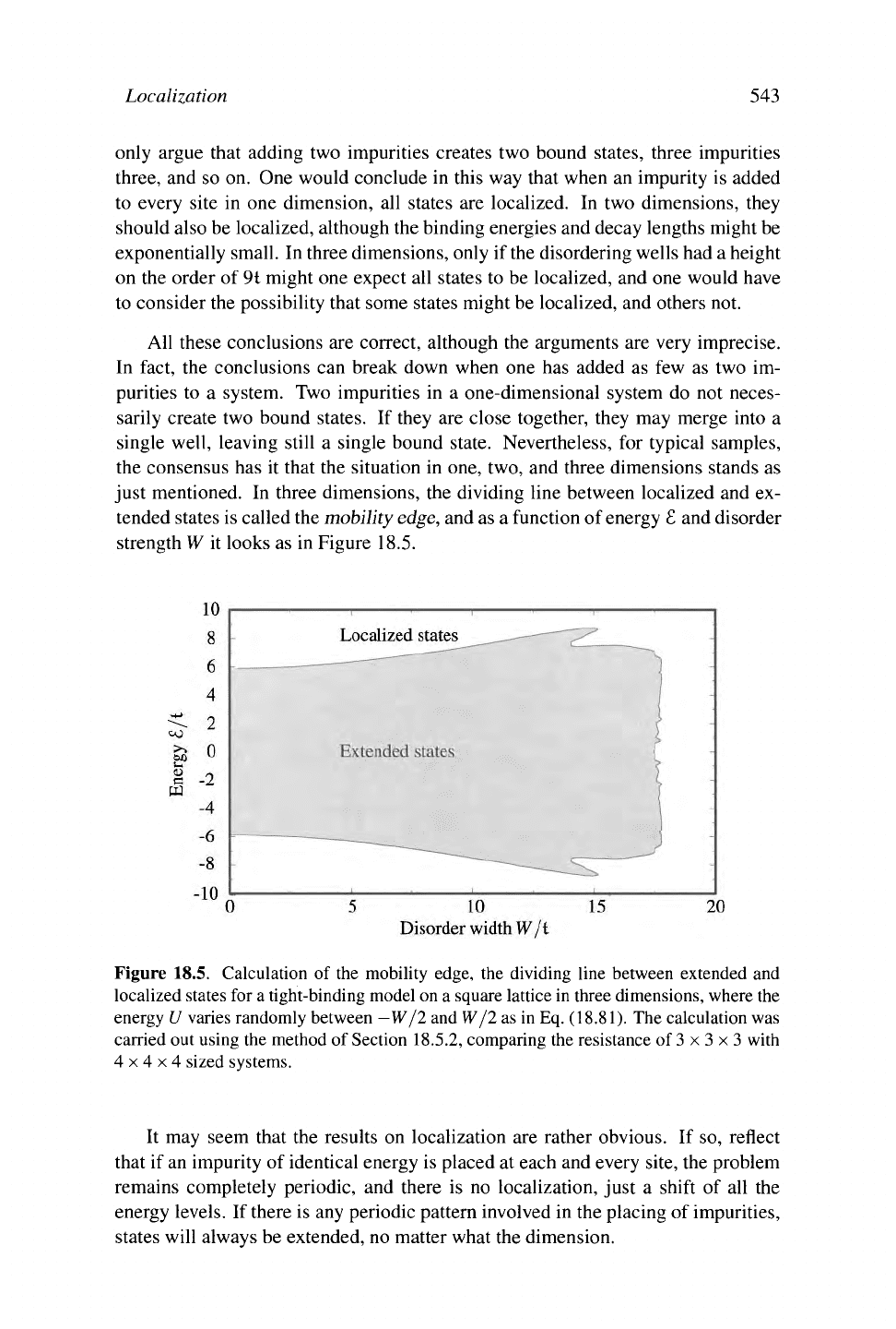
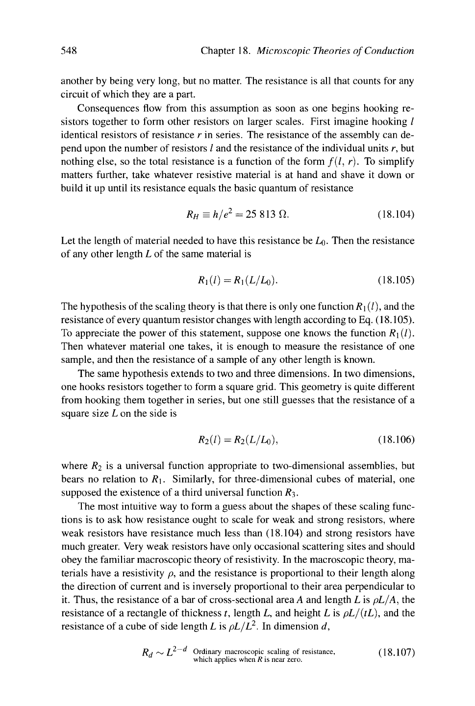
just mentioned. In three dimensions, the dividing line between localized and ex-
tended states is called the mobility
edge,
and as a function of energy £ and disorder
strength W it looks as in Figure 18.5.
Figure 18.5. Calculation of the mobility edge, the dividing line between extended and
localized states for
a
tight-binding model on a square lattice in three dimensions, where the
energy U varies randomly between
—W/2
and W/2 as in
Eq.
(18.81). The calculation was
carried out using the method of Section 18.5.2, comparing the resistance of
3
x
3
x
3
with
4x4x4 sized systems.
It may seem that the results on localization are rather obvious. If so, reflect
that if an impurity of identical energy is placed at each and every site, the problem
remains completely periodic, and there is no localization, just a shift of all the
energy levels. If there is any periodic pattern involved in the placing of impurities,
states will always be extended, no matter what the dimension.
544
Chapter 18. Microscopic Theories of Conduction
18.5.1 Exact Results in One Dimension
In the simplified setting of one spatial dimension, one can actually prove that all
states are localized and can find explicit expressions for the localization length,
which is the characteristic distance over which wave functions decay.
Consider the Hamiltonian Eq. (18.28) again. Now, however, take all the ener-
gies U
m
to be random variables, distributed with some probability 7(11). When a
specific form of 7 is needed, take
1 /W \ /W \
CP
(
[/ ) = — 01 U)6\ h £/ I
Sothe
onsite potential adopts with equal prob- (
1
g g \ )
W V2 / V 2 / ' ability all values between -W/2 and W/2.
Instead of treating the impurity potentials U
m
as small, treat the hopping matrix
element t as small instead. Then the unperturbed Green function is
(l\Go\m) = ^-; (18.82)
the overlap between adjacent sites induced by t will be the perturbation.
Definition of Localization Length. The localization length is defined to be
A
-1
= lim In |(0|G|m)|
2
, (18.83)
where the bar means that one must average over the random potentials U
m
on each
site,
using the probability distribution function 7.
In order to explain why the localization length has been defined in this manner,
it is necessary to explain the physical significance of (0\G\m) and to explain why
quantities that are easier to calculate from a formal point of view yield no physical
information.
Suppose that the eigenfunctions in the vicinity of some energy £ are localized.
This statement means that each eigenfunction is peaked somewhere in the lattice,
while away from the peak it falls off exponentially as exp[—m/A], where m is the
distance from the peak. Green's function is given by Eq. (18.35), so
<«|G(£-ntflO) = £ H^!°>. (18.84)
n
C, C
n
IT]
Because the peaks of the wave function move about randomly, only a small fraction
of the wave functions, order
1
/N where N is the number of sites in the lattice, will
be peaked at 0; the rest will be negligible because their overlap with site 0 is so
small. So
(m|G(£
-
i
V
)\0)
=V JdE'
D(£')
{
™
j^'
[
0)
(18.85)
VA
Ft ö(£)l7r(ffl|£) If the wave functions have width A, then a fraction (18.86)
N A//V have overlap of order unity with site 0, and all
the rest can be neglected.
VA
fy Z)(£)j7re e ~~
m
l Because the wave functions fall off over distance A. (18.87)
N
Localization
545
where
<fi
describes the phase of the matrix element.
The presence of the phase in Eq. (18.87) causes difficulties. When one sets
out to calculate some quantity such as electrical resistance in a disordered solid,
it is not possible analytically to carry out the calculation for any particular set of
randomly chosen energies U
m
. The only practical calculation averages over them.
The problem is that (m\G\0) is guaranteed to be zero. The phase
4>
is a random
function of the potentials U, and it will send (m\G\0) to zero on average, even
though all quantities being averaged over have the same order of magnitude. To
eliminate the problem, the localization length is defined by Eq. (18.83); squaring
the matrix element eliminates the phase problem, and taking the logarithm pulls
out 1/A.
Perturbation Theory in
Terms
of Paths. The perturbation series Eq. (18.56) has
a geometrical interpretation, in which electrons hop between sites of the lattice. In
this case, the perturbation
"K\
equals
t J2 \
l
')(
m
'l (18.88)
(I'm')
where /' and m' are nearest neighbors so Eq. (18.56) directs one to compute (l\G\m)
by summing over all paths that connect sites, n and m. The expansion is
(l\G\m) = (l\Go\m) + (l\Go £ |/i)t(mi|G
0
|ifi) +
.
. . . (18.89)
{l\m\)
Because Go is diagonal, a term in this expansion is only nonzero if
/ = l\
—>
ni\
—
h
—> nt2 ■ ■ ■ —>
m (18.90)
is a path which reaches from / to m. Each such path appears in the perturbation
expansion exactly once. For each link between two neighboring sites one puts
down a factor of t, and each time one reaches a site /' during the walk, one puts
down a factor of (/'|Go|/').
In one dimension, these formulas are particularly useful, because the number of
possible paths is so limited. For example, for
I
<m, the first nonzero contribution to
(l\G\m),
describing the amplitude for traveling from site / to site m, is the straight-
line path
(/|Go|/)t(/ + l|Go|/+l)t. ..t(m\Go\m). (18.91)
The complete expression for {l\G\m} must supplement (18.91) with higher-order
terms that involve some wiggling forward and backward before ending up at m.
Renormalized Perturbation Expansion. One can write the perturbation expan-
sion in a more compact way. The sum of all paths that begin at / and ends at m can
be constructed as the product of all paths that begin at
I
and end at I with
all
paths
that begin at / +
1
and end at
m,
but without ever coming back to I again. The re-
striction is necessary, or else the path would already have been included in the first

546
Chapter 18. Microscopic Theories
of
Conduction
set
of
paths. Denote
by
G
1
a
Green function
in
which electrons
are
forbidden
to
visit site /.
G
l
is the Green function resulting from the Hamiltonian
Ä + U
+
\m)(m\,
with
U
+
such
a
large energy that electrons
are
guaranteed
to
keep away from
m.
Then
(l\G\m)
=
(l\G\l)t{l+
\\G
l
\m).
(18.92)
However, the set of paths traveling from /
+
1
to m never visiting
/
again is the same
as the set that travels from
/ +
1
to / +
1, never visiting
/,
and then hops from
/ + 1
to
/ +
2
to
m, never visiting
/ +
1
again
(a
requirement that also rules out visiting
/
again.) Proceeding recursively in this way, one has
(/|G|m)
=
(/|G|/)t(/+l|G'|/
+
l)t(/
+
2|G
/+1
|/
+
2)
. . .
t(m\G
m
-
l
\m). (18.93)
Equation (18.93)
is
depicted schematically in Figure 18.6.
\
f ¥ f f f y
Figure 18.6. Diagram correspond-
V
il li li li M
ing to Eq. (18.93).
Inserting Eq. (18.93) into Eq. (18.83),
one
finds immediately that
to
leading
order in
1
/m,
The product
of
m terms cancels
the
factor
of
A
-l
=
_
m
n//
+
1|
t(
~/|/
+l
\n
;
moutfront.
The
first matrix element
is dif-
u
x
* * '
u
'
rerent from
all the
rest,
but its
contribution
becomes negligible as
m
—»
oo.
(18.94)
any value
of /
will do, because once the average is applied, all sites are equivalent.
Thus finding
the
localization length reduces
to
finding
the
probability
of
re-
maining
at
some site, assuming one never visits the site to the left. To evaluate this
quantity, note that the set
of
paths starting
at / +
1
and ending
at / +
1
without ever
visiting
/
consists
of
the following:
1.
The path that just stays
at / +
1
the whole time, plus
2.
Paths obtained
by
hopping
to
1
+
2, times
all
paths that
end
back
at / + 2
without touching
/ +
1,
and
finally times
all
paths that go from
/ +
1
to / + 1
without visiting
/.
In equation form,
(/
+ 1|G
/
|/ +
1)
= (/ + 1|G
0
|/ +
1)
+
=*►(/
+1|G'|/
+
1)
(/
+
1|G
0
|/+1)
xt(/
+
2|G
,+1
|/
+
2)
xt(/+l|G'|/
+ l)
(18.95)
1
Using Eq.
(
18.82);
see (18 96)
£-[//+l-t
2
(/ + 2|G
/
+
1
|/ + 2)' Figure 18.7.
Because
all
sites
are
equivalent, take
/ = 0. The
probability distribution
of
(1
|tG°|
1)
can now
be
obtained from the probability distribution J
5
for [//.
All one
Localization 547
\w
= 0 _|_ \t \y
Figure 18.7. Diagram correspond-
*
^»CV
ing to Eq. (18.96).
needs
is
Eq. (18.96). The probability
3
that tG° will adopt some value
g is
^(S>
£
)= fl[[dU
m
nU
m
Mg-(\\tG
0
(e.)\\))
(18-97)
=
[
Y\[dU
m
7(U
m
)]S(g
; )
Use
Eq.
(18.96).
(18.98)
J
V
V ;J
\ £-f/,-t
2
(2|G
1
|2)>'
=
/4
n^
(/
-
:P
(
f/
'»)]
;P
(
£
---
t2
<
2
l
0
'!
2
))
(
18
-")
J
g
m+\
8
The only appearance
of
U\
is now
made explicit,
so one can
integrate over
it.
Next, reintroduce the integral over
U\
to
find....
=
4 /
Y[[dU
m
y{U
m
)}
j
dg'
?(£ - --ig')s(g'-t(2\G
l
|2))
(18.100)
= \ i dg' 0>(£ - - -ig') ?(g', £). Thelasttermin (18.101)
P
z
J V g / Eq. (18.100) just gives the
In general, the integral equation (18.101) must be solved numerically, but in the
limit
of
weak disorder, where the standard deviation
of
the distribution
CP
is
much
smaller than
t,
one can obtain definite results. The details are assigned
to
problem
8, and the result is that
for £ = 0
M
2
A"
1
=0.1142—. (18.102)
When the probability distribution takes the form
of
Eq.
(18.81),
105.045t
2
A=
. W is
the width
of
the disorder. (18.103)
W
2
18.5.2 Scaling Theory
of
Localization
The most powerful theory
of
localization
is a
scaling theory
of
Abrahams
et al.
(1979).
It bypasses the obvious sort of calculation, such as extracting conductivities
from some microscopic model,
and
instead derives advantage from
a
deceptively
simple physical postulate. The resulting theory provides
a
framework
in
which
to
organize theoretical, numerical, and experimental data.
The physical idea behind
the
scaling theory
is
very simple. Suppose
one has
a
bag
filled with resistors. Assume that
no
matter
how one
hooks
the
resistors
together, any two with the same resistance are indistinguishable. One resistor might
obtain
its
large resistance from
a
small density
of
states, another
by
having
the
Fermi energy
sit
near
the
band edge, another
by
being very highly disordered,
548
Chapter 18. Microscopic Theories of Conduction
another by being very long, but no matter. The resistance is all that counts for any
circuit of which they are a part.
Consequences flow from this assumption as soon as one begins hooking re-
sistors together to form other resistors on larger scales. First imagine hooking /
identical resistors of resistance r in series. The resistance of the assembly can de-
pend upon the number of resistors / and the resistance of the individual units r, but
nothing else, so the total resistance is a function of the form /(/, r). To simplify
matters further, take whatever resistive material is at hand and shave it down or
build it up until its resistance equals the basic quantum of resistance
R
H
= h/e
2
= 25 813 O. (18.104)
Let the length of material needed to have this resistance be
LQ.
Then the resistance
of any other length L of the same material is
R
X
[1)=R
X
{L/L
Q
).
(18.105)
The hypothesis of
the
scaling theory is that there is only one function R\ (I), and the
resistance of every quantum resistor changes with length according to Eq. (18.105).
To appreciate the power of this statement, suppose one knows the function R\ (I).
Then whatever material one takes, it is enough to measure the resistance of one
sample, and then the resistance of a sample of any other length is known.
The same hypothesis extends to two and three dimensions. In two dimensions,
one hooks resistors together to form a square grid. This geometry is quite different
from hooking them together in series, but one still guesses that the resistance of a
square size L on the side is
R
2
(l)=R
2
{L/Lo),
(18.106)
where R
2
is a universal function appropriate to two-dimensional assemblies, but
bears no relation to R]. Similarly, for three-dimensional cubes of material, one
supposed the existence of a third universal function Rj,.
The most intuitive way to form a guess about the shapes of these scaling func-
tions is to ask how resistance ought to scale for weak and strong resistors, where
weak resistors have resistance much less than (18.104) and strong resistors have
much greater. Very weak resistors have only occasional scattering sites and should
obey the familiar macroscopic theory of resistivity. In the macroscopic theory, ma-
terials have a resistivity p, and the resistance is proportional to their length along
the direction of current and is inversely proportional to their area perpendicular to
it. Thus, the resistance of a bar of cross-sectional area A and length L is pL/A, the
resistance of a rectangle of thickness t, length L, and height L is pL/{tL), and the
resistance of a cube of side length L is pL/L
2
. In dimension d,
R, r^ L Ordinary macroscopic scaling of resistance, (18.107)
which applies when R is near zero.
Localization
549
must give the behavior of R
d
when R is close to zero. Conversely, when R is very
large, one should expect all states to be localized and should also expect R to rise
exponentially with sample length as
/^ r^j (AdL/Lo A
d
j
s
some
dimensionless constant depending (18.108)
upon dimensionality.
In d
— 1
and d = 2, there is no problem supposing that R rises monotonically with
L.
However, in d = 3, R shrinks as a function of L when it is small, and it grows
when it is large. Rather than making guesses about the shapes of Rd, Abrahams
et al. (1979) proposed that one focus on the functions
a
,
v
. LÖR d\nR dlnR
d
{L/Lo)
ßd{R) =
RdL
=
^L
=L
dl
(18.109)
and guessed that ßd(R) is a smooth, monotonically increasing function. That
is,
the
change of resistors with scale increases continuously as their resistance increases.
This guess is not obvious, and it emerged in part as a compact way to sum up a
variety of seemingly disconnected theoretical results. It is at least consistent with
their asymptotic behavior. For resistors R near zero,
ß
d
(R)~2-d,
From Eq. (18.107).
(18.110)
while for large R
ß
d
{R)~
— ~\n R.
LQ
A schematic view of ßd(R) appears in Figure 18.8.
6 I j "T. 5
4
a;
e
CO
-J
c
CO
II
oe,
en
3.
2
U
-2
(A)
1-d ^^^/
2-d ___^^
3-d __^~^
-5
0
In/?
(18.111)
-5 0
ln(L/Lo)
Figure 18.8. (A) Sketch of qualitative behavior of the three functions ßd{R), given the
asymptotic behavior in Eqs. (18.110) and (18.111) and assuming smooth interpolation be-
tween these two limits. (B) Three scaling functions In R versus In L/LQ resulting from
the three functions ß. At the point where the three-dimensional ß function crosses 0, the
resistance has a logarithmic singularity.
550
Chapter 18. Microscopic Theories of
Conduction
In one dimension, ß is a smooth positive function. In two dimensions, it is
always positive, but approaches zero along the negative In R axis. In three dimen-
sions,
ß must cross through zero. As a result, the scaling functions
. r d In R The point of
this
expression is to view In L/LQ
ln(L/L()j= / — as a function of In /?, and guess the shape of (18.112)
J ßd\}
n
R) this function by guessing that ß
d
(\n R) has
the form shown in Figure 18.8.
have singularities in two and three dimensions. In two dimensions the singularity
occurs for R
—>
0, while in three dimensions it occurs at a finite value of R. In
two dimensions, the prediction of Figure 18.8 is that the larger a system gets, the
larger its resistance gets. In other words, in the macroscopic limit, all states in
two dimensions should be localized. In three dimensions the prediction is that
for resistance below a universal critical value, making a system larger continually
reduces its resistance, while for any system with resistance above this critical value,
making it larger makes the resistance grow. The scaling theory recovers in this way
the prediction of
the
mobility edge, and furthermore it states that to know whether a
system lies on the localized or extended side of the edge, it is sufficient to measure
its resistance at any scale.
These scaling ideas are particularly well suited to guide interpretation of nu-
merical work. It would seem easy to investigate localization numerically. All one
has to do is to write down a Hamiltonian with randomly chosen diagonal matrix el-
ements, calculate the eigenfunctions, and classify them according to whether they
are localized or extended. There is in fact no difficulty in carrying out such a calcu-
lation for lattices on the order of 13 x 13 x 13. However, the results are extremely
difficult to interpret. As the degree of randomness increases, the eigenfunctions all
become bumpier and bumpier in a continuous way. There is no sign of a transition
at some value of randomness, and there is no simple function that can be applied
to the randomly oscillating wave functions to indicate whether they can carry cur-
rent or not. In an infinite system, localized wave functions rise above zero only in
the neighborhood of a limited number of lattice sites, but for the relatively small
systems that can be solved numerically, localization is not visible.
Using the ideas of the scaling theory produces a completely unambiguous de-
termination of localization. Rather than examining the properties of any single
wave function or any single Hamiltonian, attention shifts to how the solutions alter
with change of scale.
Figure 18.9 illustrates the process for a cubic lattice in three dimensions, de-
scribed by Eq. (18.28) and with the the probability distribution of impurity poten-
tials described by Eq. (18.81). Problems 5 through 7 describe how to compute
its resistance. Fluctuations of resistance are extremely large from one sample to
another. Indeed, they are so large that R, the average of resistance over many re-
alizations of the disorder, cannot be computed. A criterion for determining when
such an average has converged is that 6R
2
= R
2
—
R should fall below some speci-
fied tolerance. When monitoring SR
2
, one will find that it never converges to zero.
l2
However, In R does converge; [In R]
2
—
In R can be made as small as desired by
Localization
551
Figure 18.9. Three-dimensional scaling function for square lattice with diagonal disorder.
(A) In R/Rfj
(RH
= h/e
2
) is plotted versus In L for systems ranging from 2
3
to 7
3
in size,
and disorder W ranging from 0 to 20. The transition from localized to extended states
occurs around
IV
= 17. (B) Each curve is displaced horizontally so as to overlap with the
other
curves,
forming the scaling function R^L/LQ).
sampling enough systems. An additional reason to define the localization length as
in Eq. (18.83) is that Green's functions fluctuate too much for their averages to be
well-defined, but averages of logarithms converge.
Figure 18.9(A) shows plots of In R as a function of
In
L. Averages over around
10
5
systems are required to obtain 1% accuracy. According to the basic scaling
hypothesis, for any given level of disorder W, In R versus In L should lie on a
universal curve once L is appropriately scaled, meaning that each curve in Figure
18.9(A) must be shifted horizontally until it touches the curve below. The result
is displayed in Figure 18.9(B), which shows the universal function
Rj(l).
There
is a transition between metals and insulators at a disorder W of around 17. If the
disorder is larger than this critical value, resistance increases continually with L,
and macroscopic samples of the material must be insulating. If the disorder is less,
resistance decreases with sample size, and the material is a metal. The distinction
between metals and insulators is apparent in very small systems; one can distin-
guish between them by monitoring the change in In R when passing from 2x2x2
systems to 3 x 3 x 3 systems. Figure 18.5 shows the result of comparing In R for
800 values of W and £, for systems of size 3x3x3 and 4x4x4, identifying
localized states as those where the resistance increases for the larger system, and
identifying extended states as those where it decreases.
18.5.3 Comparison with Experiment
According to Figure 18.9, the resistance of an insulating solid grows exponentially
as its size increases. Two 30 000 Ü resistors hooked in series should give much
more than 60000 Q. These predictions are of course false. Macroscopic resistors
552
Chapter 18. Microscopic Theories of Conduction
10
3
S
o
■% 10
1
at,
10
4
_ 10
3
I
102
"S.
10'
1
/ -
/ '
► y -.
~~~—*-~~^^
s
^
(A)
10
100 10"
5
10"
4
10"
3
10"
2
10-' 1
Temperature T (K) (B) l
T
oc T"
0325
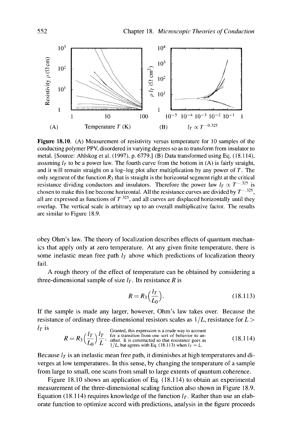
Figure 18.10. (A) Measurement of resistivity versus temperature for 10 samples of the
conducting polymer PPV, disordered in varying degrees so as to transform from insulator to
metal. [Source: Ahlskog et al. (1997), p. 6779.] (B) Data transformed using Eq. (18.114),
assuming lj to be a power law. The fourth curve from the bottom in (A) is fairly straight,
and it will remain straight on a log-log plot after multiplication by any power of T. The
only segment of the function
/?3
that is straight is the horizontal segment right at the critical
resistance dividing conductors and insulators. Therefore the power law lj oc
T~
325
is
chosen to make this line become horizontal. All the resistance curves are divided by
T~
325
,
all are expressed as functions of
T
325
,
and all curves are displaced horizontally until they
overlap. The vertical scale is arbitrary up to an overall multiplicative factor. The results
are similar to Figure 18.9.
obey Ohm's law. The theory of localization describes effects of quantum mechan-
ics that apply only at zero temperature. At any given finite temperature, there is
some inelastic mean free path lj above which predictions of localization theory
fail.
A rough theory of the effect of temperature can be obtained by considering a
three-dimensional sample of size lj. Its resistance R is
R
Mh)
(18.113)
If the sample is made any larger, however, Ohm's law takes over. Because the
resistance of ordinary three-dimensional resistors scales as 1/L, resistance for L >
IT is
R = R3
. . Granted, this expression is a crude way to account
lj \ lj f
or a
transition from one sort of behavior to an-
~f~ j
~j~
■
other. It is constructed so that resistance goes as
^O
L
1/L, but agrees with Eq.
( 18.113)
when l
T
= L.
(18.114)
Because lj is an inelastic mean free path, it diminishes at high temperatures and di-
verges at low temperatures. In this sense, by changing the temperature of a sample
from large to small, one scans from small to large extents of quantum coherence.
Figure 18.10 shows an application of Eq. (18.114) to obtain an experimental
measurement of the three-dimensional scaling function also shown in Figure 18.9.
Equation (18.114) requires knowledge of the function lj. Rather than use an elab-
orate function to optimize accord with predictions, analysis in the figure proceeds