Middleton W.M. (ed.) Reference Data for Engineers: Radio, Electronics, Computer and Communications

28-1

2

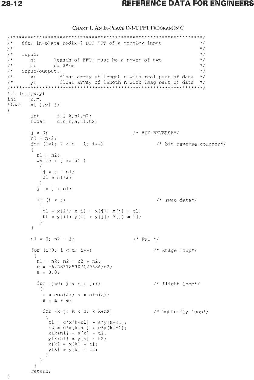
CHART

1.

AN

IN-PLACE

D-I-T

FFT

PROGRAM IN

C

....................................................................

/*

fft: in-place radix-2 DIT DFT of a complex inp-ct

*/

/* */

/*

input:

*/

/*

n:

length

of

FFT: must be

a

power of two

*/

/*

m:

n=

2**m

*/

/*

input/output:

*/

/*

x:

float array

of

length

n

with real part of data

*/

/*

Y:

float array

of

length

n

with imag part of data

*/

....................................................................

fft

in,m,x,y)

int

n,m;

float

x[ 1,y

I

int

float

j

=

0;

n2

=

n

I;

i

,

j

,

k,

nl

,

n2

;

c, s, e, a, tl, t2;

for

(i=l;

1

<

n

-

1;

i++)

{

nl

=

n2;

while

(

j

>=

nl

j

I

j

=

j

-

nl;

nl

=

11112;

j

=

j

+

nl;

}

/*

BIT-REVERSE*/

/*

bit-reverse counter*/

if

(i

i

j)

/*

swap d.ata*/

I

tl

=

x[il; x[il

=

x[jl;

x[jl

=

tl;

tl

=

y[il;

y[il

=

y[jl;

Y[jl

=

tl;

1

}

nl

=

0;

n2

=

1;

/*

FFT

*/

for (i=O; i

<

m; i++)

I

nl

=

n2;

n2

=

n2

+

n2;

e

=

-6.283185307179586/112;

a

=

0.0;

for

(j=O;

j

i

nl;

j++)

I

c

=

cos(aj;

s

=

sin(aj;

a=a+e;

for

(k=j;

k

<

n;

k=k+n2)

I

tl

=

c*x[k+nll

-

s*y[k+nll;

t2

=

s*x[k+nll

+

c*y[k+nl];

x[k+nlI

=

x[kl

-

tl;

y[k+nll

=

y[k]

-

t2;

x[kl

=

~[kl

+

tl;

~[kl

=

~[kl

+

t2;

1

/*

stage

loop*/

/*

flight

loop*/

/*

butterfly loop*/

1

return;

1

DISCRETE-TIME SIGNAL PROCESSING

28-1

3

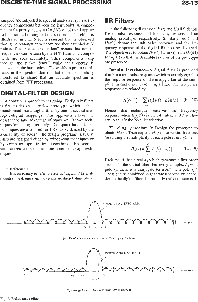
sampled and subjected to spectral analysis may have fre-

quency components between the harmonics.

A

compo-

nent at frequency

wk+1,2

=

(2~

/

N)(k

+

%)

will appear

to be scattered throughout

the

spectrum. The effect is

illustrated in Fig.

5

for a sinusoid that is observed

through a rectangular window and then sampled at

N

points. The “picket-fence effect” means that not all

frequencies can be seen by the FFT. Harmonic compo-

nents are seen accurately. Other components “slip

through the picket fence” while their energy is

“leaked” in the harmonics.* These effects produce arti-

facts in the spectral domain that must be carefully

monitored

to

assure that an accurate spectrum is

obtained from FFT processing.

DIG

ITAL-

FI

LTE

R

D

ESI

G

N

A

common approach to designing

IIR

digital? filters

is first to design an analog prototype, which is then

transformed into a digital filter by one of several ana-

log-to-digital mappings. This approach allows the

designer to take advantage of many well-known tech-

niques for analog-filter design. Computer-based design

techniques

are

also used for

IIRS,

as evidenced by the

availability of several

IIR

design programs. Usually,

FIRS

are designed either by windowing techniques

or

by computer optimization algorithms. This section

summarizes some of the more common design tech-

niques.

*

Reference

3.

t

It is customary to refer

to

these as “digital” filters,

al-

though at the design stage they really

are

discrete-time filters.

IIR

Filters

In

the following discussion,

h,(t)

and

H,(isz)

denote

the impulse response and frequency response of

an

analog prototype, respectively. Similarly,

h(n)

and

H(d”)

denote

the

unit pulse response and the fre-

quency response of the digital filter to be designed.

The objective is to obtain

H(d”)

(or

h(n))

from

Ha(@)

(or

h,(t))

so

that the desirable features of the prototype

are preserved.

Impulse

Invariance-A

digital filter is produced

that has a unit pulse response which is exactly equal

to

the impulse response of the analog filter at the

sam-

pling instants; i.e.,

h(n)

E

h,(t)lt=,zp

The frequency

responses

are

related by

+oa

Hence, this technique preserves the frequency

response when

HJj(i2)

is band-limited, and

T

is cho-

sen

to

satisfy the Nyquist criterion.

The design procedure

is:

Design the prototype to

obtain

Ha($).

Then expand HJs) into partial fractions

(assuming the multiplicity of each pole is unity), i.e.

Each real

A,

has a real

sk,

which generates a first-order

section in the digital filter. For every complex

A,

with

pole

sk,

there is a conjugate term

A&*

with pole

sk*

These can be combined to generate a second-order sec-

tion

in

the digital filter that has only real coefficients. If

‘’\

UNDERLYING

SPECTRUM

/I\

(A)

FFT

of

a

wlndowed sinusoid with frequency

ok

=

Zlrk/N

(BJ

Leakage

for

a

nonharmonlc

sinusoldal

component

Fig.

5.

Picket-fence effect

28-1

4

REFERENCE

DATA

FOR ENGINEERS

there are

M

real poles and

L

complex conjugate pairs,

the resulting digital filter becomes

where

a,

=

A,

(real)

b

-

+a/T

1-

cm

=

-2T

Re

{

Ak

}

ckl

=

-2T

e"k7

Re{

A,

e-joJcT

I

d

k2

- -

e2akT

dkl

=

-2

eakT

cos

(&T)

(Eq. 21)

and

sk

=

aik

+

j

Pk

is the k%h pole of

H,(s).

Note that

H(z)

is completely defined in terms of

ak,

sk,

and

T.

Features:

(I)

Good only for band-limited

Ha($).

(2)

Results initially in a parallel form.

(3)

O

=

QT

-+

linear relationship between the ana-

log and digital frequency variables.

(4)

The impulse invariant technique is not an alge-

braic mapping; i.e.,

H(z)

cannot be obtained

from

HJs)

by a substitution of variable.

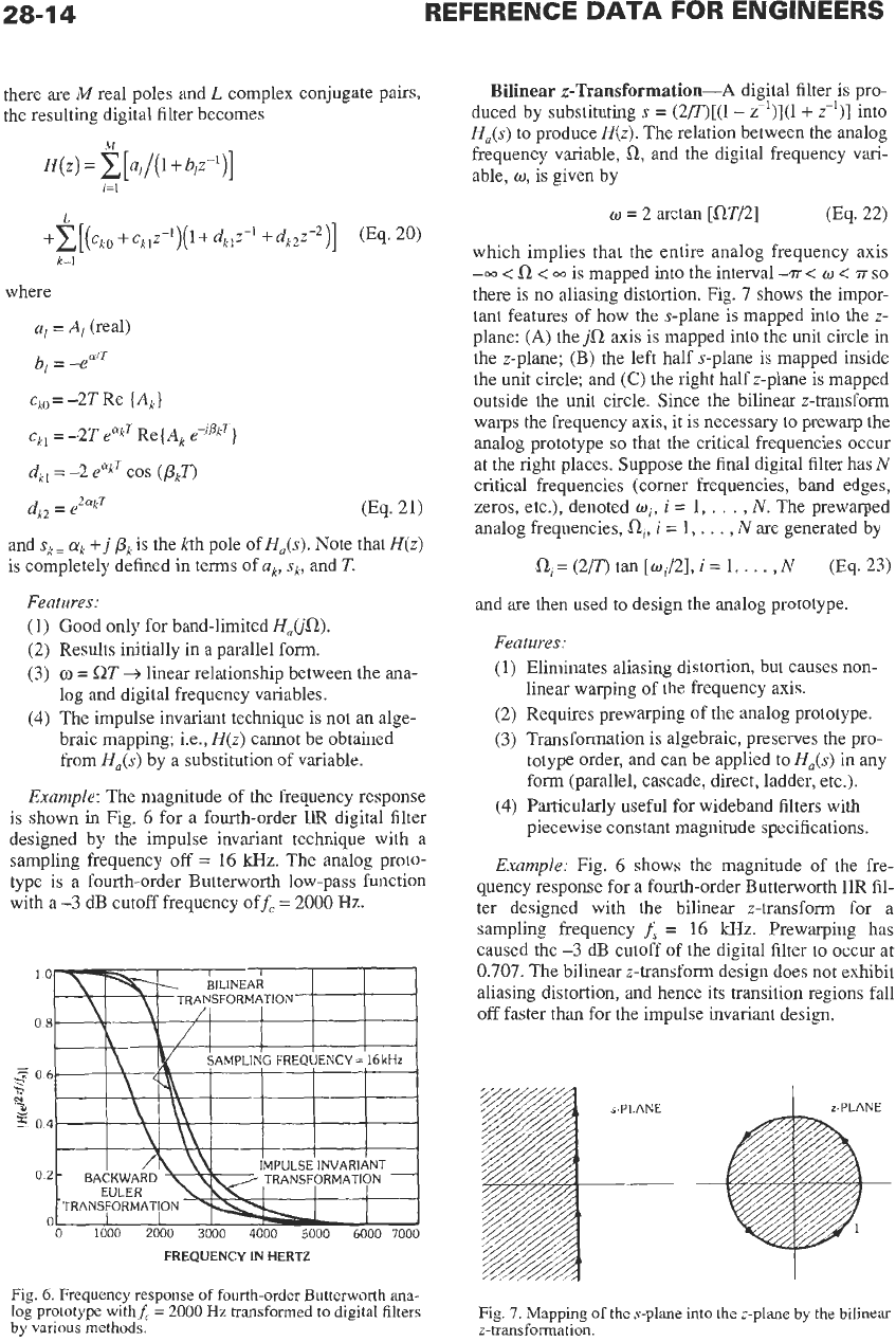
Example:

The magnitude of the frequency response

is shown in Fig. 6 for a fourth-order LIR digital filter

designed by the impulse invariant technique with a

sampling frequency off

=

16

kHz.

The analog proto-

type is a fourth-order Butterworth low-pass function

with a

-3

dB cutoff frequency off,

=

2000

Hz.

0

1000

2000

3000

4000

5000

6000

7000

FREQUENCY IN HERTZ

Fig.

6.

Frequency response

of

fourth-order Butterworth ana-

log prototype withf,

=

2000

Hz

transformed to digital filters

by

various

methods.

Bilinear z-Transformation-A

digital filter

is

pro-

duced by substituting

s

=

(2/T)[(1

-

z-')](l

+

z-')]

into

H,(s)

to

produce

H(z).

The relation between the analog

frequency variable,

a,

and the digital frequency vari-

able,

o,

is given by

o

=

2

arctan

[aT/2]

(Eq.

22)

which implies that the entire analog frequency axis

--w

<

a<

-

is mapped into the interval

-T

<

w

<

T

so

there

is

no aliasing distortion. Fig.

7

shows the impor-

tant features of how the s-plane is mapped into the

z-

plane:

(A)

the

ji2

axis is mapped into the unit circle in

the z-plane; (B) the left half s-plane is mapped inside

the unit circle; and

(C)

the right half z-plane is mapped

outside the unit circle. Since the bilinear z-transform

warps the frequency axis, it is necessary to prewarp the

analog prototype

so

that the critical frequencies occur

at the right places. Suppose the final digital filter has

N

critical frequencies (corner frequencies, band edges,

zeros, etc.), denoted

mi,

i

=

1,

.

. .

,

N.

The prewarped

analog frequencies,

ai,

i

=

1,

. . .

,

N

are generated by

a,

=

(2/T)

tan

[wi/2],

i

=

1,

. .

.

,

N

and are then used to design the analog prototype.

(Eq. 23)

Features:

(1) Eliminates aliasing distortion, but causes non-

(2) Requires prewarping of the analog prototype.

(3) Transformation is algebraic, preserves the pro-

totype order, and can be applied to

H,(s)

in any

form (parallel, cascade, direct, ladder, etc.).

(4)

Particularly useful for wideband filters with

piecewise constant magnitude specifications.

Example:

Fig.

6

shows the magnitude of the fre-

quency response for a fourth-order Butterworth IIR fil-

ter designed with the bilinear z-transform for a

sampling frequency

f,

=

16

IcHz.

Prewarping has

caused the

-3

dB cutoff of the digital filter to occur at

0.707.

The bilinear z-transform design does not exhibit

aliasing distortion, and hence its transition regions fall

off

faster than for the impulse invariant design.

linear warping of the frequency axis.

Fig.

7.

Mapping

of

the s-plane into the z-plane by the bilinear

z-transformation.

DISCRETE-TIME

SIGNAL

PROCESSING

28-1

5

Euler Transformations-Although the Euler trans-

formations are,

in

general, inferior to the above two

design techniques for digital filters, they

are

mentioned

here because they occur frequently for the discrete-

time solution

of

differential equations. The backward

and forward Euler transformations

are

algebraic trans-

formations characterized in the frequency domain by

s

=

(1/T)(l

-

z-')

and

s

=

(l/T)(z

-

1),

respectively. The

backward Euler transformation results from a back-

ward difference approximation to the first derivative,

whereas the forward Euler transformation results from

a forward difference approximation.* Both of the

Euler transformations are known to distort the fre-

quency response unless the sampling rate is very high

with respect to the upper band edge of the analog pro-

totype. The backward Euler transformation always

maps stable analog prototypes into stable digital fil-

ters.

In

contrast,

the

forward Euler transformation has

the potential to map a stable prototype into

an

unstable

digital filter unless the sampling rate is chosen suffi-

ciently high.

In

Fig.

6,

a backward Euler design for the fourth-

order Butterworth

IIR

example is shown for the

sam-

pling ratef,

=

16

Wz. It

is

apparent that the backward

Euler design results

in

considerable distortion

in

com-

parison with the other two designs.

Nonlinear Optimization Methods-Digital filter

design techniques exist which treat the design

as

a

nonlinear optimization problem.

In

particular, Dec-

zky's method is often used.? Nonlinear design meth-

ods are more complicated

than

transformation of an

analog prototype filter via the methods described

above. However, direct nonlinear optimization allows

much more freedom in the frequency responses that

are designed and the accompanying optimization crite-

ria.

FIR

Filters

Two general approaches are available for the design

of FIR digital filters:

(1)

designs by windowing tech-

niques and

(2)

optimal designs by computer optimiza-

tion

techniques.

In

general, window designs can be

carried out with the aid of a hand calculator and a table

of well-known window functions.

In

contrast, com-

puter optimization requires a sophisticated computer

program and a considerable amount of computer time.

Filters obtained by method

2

are, in general, higher

quality filters. Also, more elaborate filter specifications

can be approximated because the computer does most

of the work.

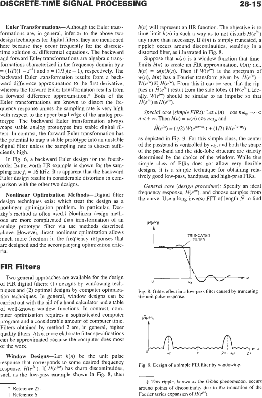
Window Designs-Let

h(n)

be the unit pulse

response that corresponds to some desired frequency

response,

H(eim).

If

H(eJ")

has sharp discontinuities,

such

as

the low-pass example shown

in

Fig.

8,

then

-

*

Reference

25.

t

Reference

6

h(n)

will represent an

IIR

function. The objective is to

time-limit

h(n)

in

such a way

as

to not disturb

H(d")

any more than necessary. If

h(n)

is simply truncated,

a

ripple4 occurs around discontinuities, resulting in a

distorted filter, as illustrated

in

Fig.

8.

Suppose that

w(n)

is a window function that time-

limits

h(n)

to

create an

FIR

approximation,

h(n);

i.e.,

h(n)

=

w(n)h(n).

Then if

W(d")

is the specpm of

w(n),

h(n)

has a Fourier transform given by

N(d")

=

W(d")

O_

H(d").

From this it can be seen that the rip-

ples in

H(dW)

result from

the

side lobes

of

W(dw).

Ide-

aily,

W(e'"')

should be similar to an impulse

so

that

Special case (simple

FIRS):

Let

h(n)

=

cos

nuo,

-

<

H(d")

EH(d").

n

<

+

m.

Then

h(n)

=

o(n)

cos

nw,,

and

$P)

=

(1~)

w(P+"o)

+

(1/2)

W(e'*"O>

as depicted in Fig.

9.

For this simple class, the center

of the passband is controlled by

coo,

and both the shape

of the passband and the side-lobe structure

are

strictly

determined by the choice of the window. While this

simple class of

FIRS

does not allow very flexible

designs, it is a simple technique for obtaining rela-

tively good low-pass, bandpass, and high-pass

FIRS.

General case (design procedure):

Specify an ideal

frequency response,

H(e""),

and choose sampies from

the curve. Use a long inverse

FFT

of length

N

to

find

1

H(dw)

I

TRUNCATED

,

FlLTER

Fig.

8.

Gibbs

effect

in

a

low-pass

filter

caused

by

truncating

the

unit

pulse

response.

Fig.

9.

Design

of

a

simple

FIR

filter

by

windowing.

$

This

ripple,

known

as

the

Gibbs

phenomenon,

occurs

around

points

of

discontinuity

due

to

the

truncation

of

the

Fourier

series

expansion

of

~(ei").

28-1

6

REFERENCE

DATA

FOR ENGINEERS

an approximation

io

h(n),

where

ifN

is the desired length

of the

HR,

then

N

>>

N.

Then use a carefully selected

window to truncate

h(n)

according to

hjn)

=

w(n)lz(n).

Finally, use an

FFT

of length

N

to find

H(d”).

If

h(dw)

is a satisfactory approximation to

H(dw),

the design is

finished. If not, choose a new

H(dw)

or a new

o(n)

and

repeat. Throughout the procedure, it is important to

choose

N

=

W,

with

k

an integer in the range [4,

.

. .

,

101.

The

k

should be made as large as possible within

the limits of the computer resources. This design tech-

nique is

a

trial-and-error procedure. The quality

of

the

result will depend to some degree on the skill and

experience of the designer.

Table 4 lists a few well-known window functions

that can be used in this procedure. An extensive list of

windows and their figures of merit has been published

in Reference

12.

Computer Design

by

Equiripple Approxima-

tion-There are quite a few publications and numer-

ous

computer programs that deal with optimized

designs for

FIRS

using equiripple approximations in

the frequency domain. One popular program that has

been widely distributed is the one published by

McClellan, et. al.* This program is capable of design-

ing bandpass (including low-pass and high-pass), dif-

ferentiator, and Hilbert-transform

FIR

filters under the

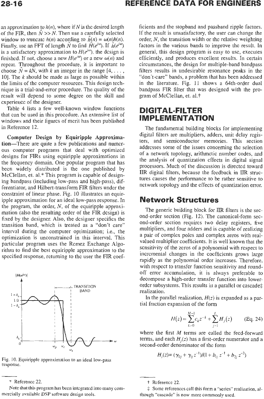
constraint of linear phase. Fig.

10

illustrates an equir-

ipple approximation for an ideal low-pass response.

In

the program, the order,

N,

of the equiripple approxi-

mation (also the resulting order

of

the FIR design) is

fixed by the designer. Also, the designer specifies the

transition band, which is treated as a “don’t care”

interval during the computer optimization; Le., the

optimization is unconstrained in this interval. This

particular program uses the Remez Exchange Algo-

rithm to find the best equiripple approximation to the

specified response, returning to the user the FIR coef-

10

1

-

6,

6

w

Fig.

10.

Equiripple approximation to an ideal low-pass

response.

*

Reference

22.

Note that this program has been integrated into many com-

mercially available

DSP

software design tools.

ficients and the stopband and passband ripple factors.

If the result is unsatisfactory, the user can change the

order,

N,

the transition width or the relative weighting

factors in the various bands to improve the result.

In

general, this design program is easy to use, executes

efficiently, and produces excellent results.

In

certain

circumstances, the design for multiple-band bandpass

filters results in undesirable resonance peaks

in

the

“don’t-care’’ bands, a problem that has been addressed

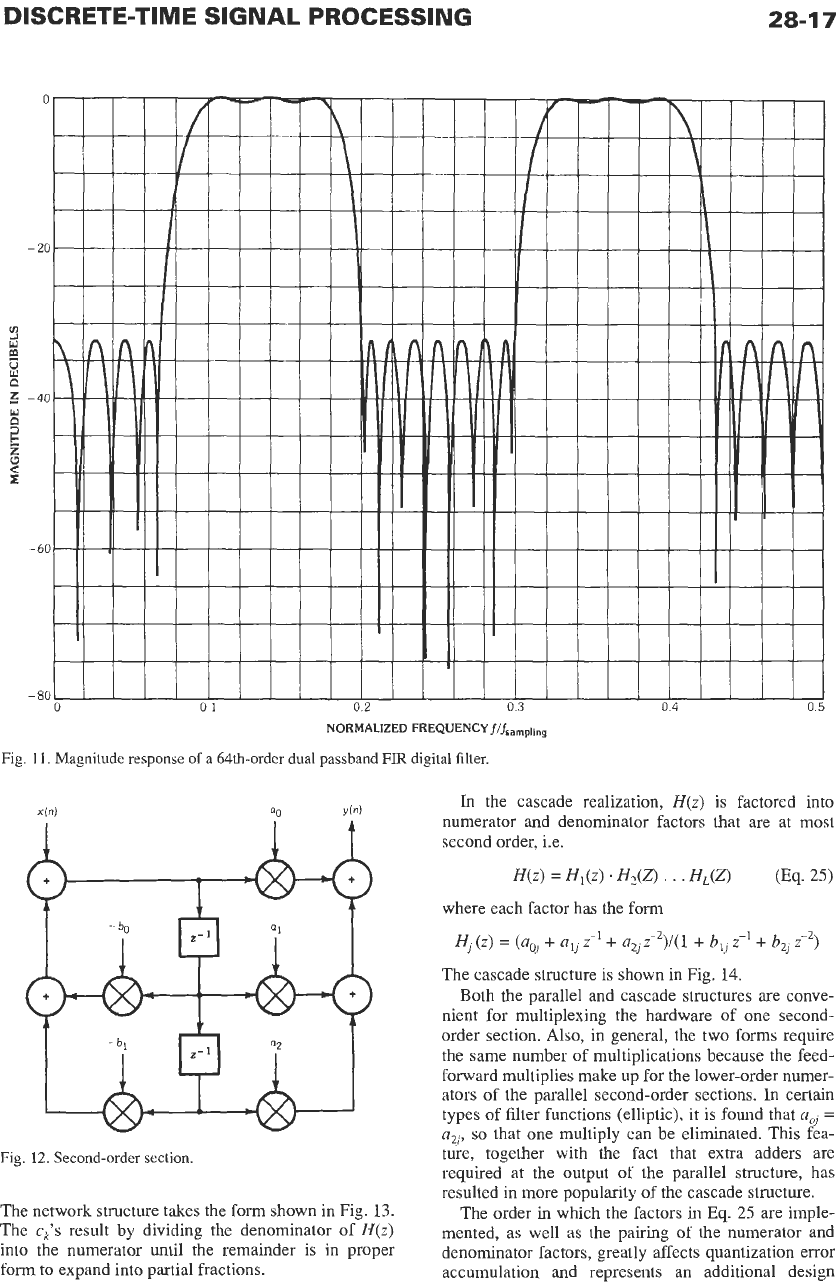
in the literature. Fig.

11

shows a 64th-order dual

bandpass FIR filter that was designed with the pro-

gram of McClellan,

et.

al.?

DIG

ITAL-FI LTE

R

IMPLEMENTATION

The fundamental building blocks for implementing

digital filters are multipliers, adders, unit delay regis-

ters, and semiconductor memories.

This

section

addresses some of the issues concerning the selection

of a network topology, arithmetic number codes, and

the analysis of quantization effects in digital signal

processors. Much of the discussion is directed toward

IIR

digital filters, because the feedback

in

W

struc-

tures causes the performance to be rather sensitive to

network topology and the effects of quantization error.

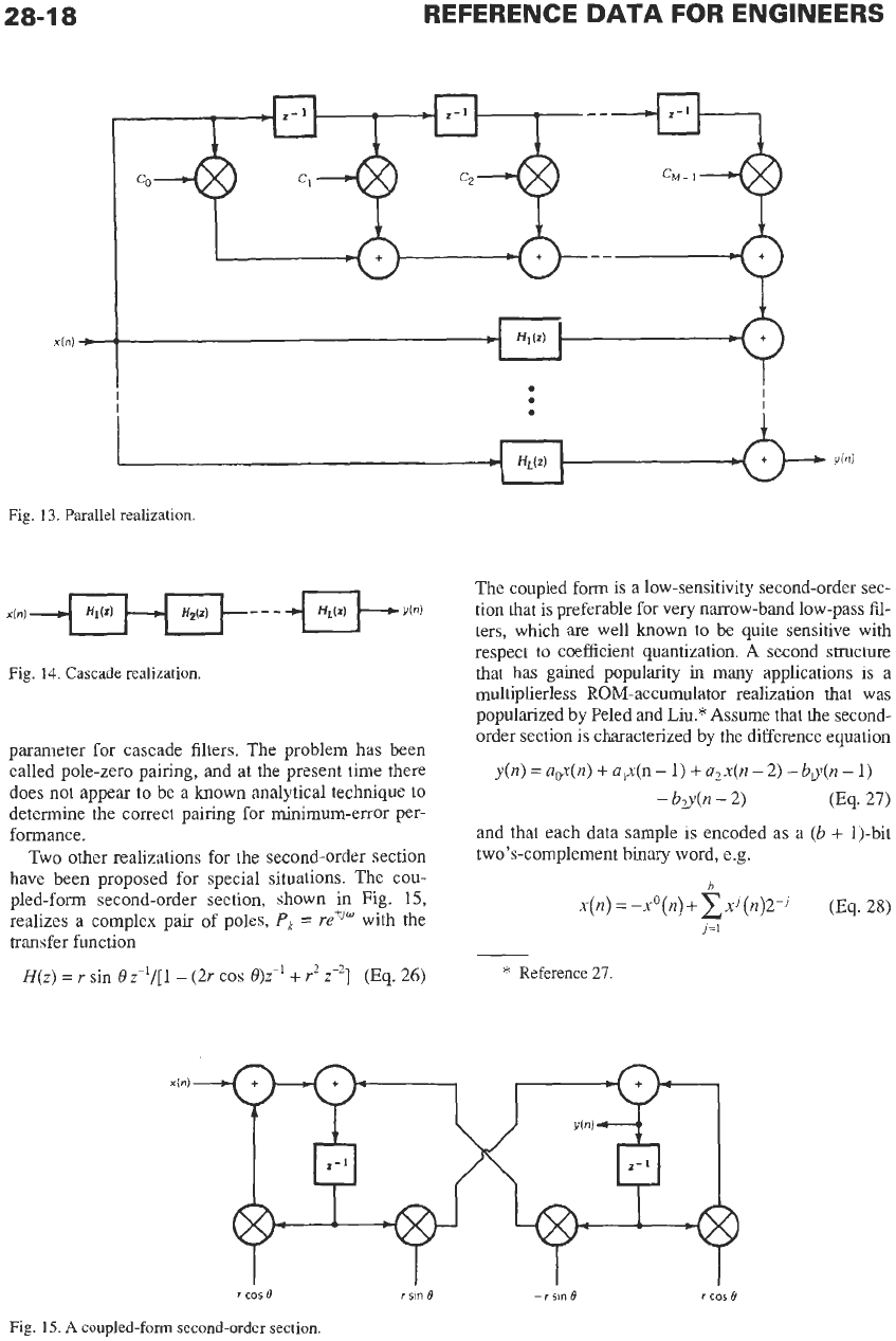
Network Structures

The generic building block for

IIR

filters is the sec-

ond-order section (Fig.

12).

The canonical-form sec-

ond-order section requires two delay registers, five

multipliers, and four adders and is capable of realizing

a pair of complex poles and complex zeros with real-

valued multiplier coefficients.

It

is

well known that the

sensitivity of the zeros of a polynomial with respect to

incremental changes in the coefficients grows large

rapidly as the polynomial order increases. Therefore,

with respect to transfer function sensitivity and round-

off error accumulation,

it

is always preferable

to

decompose a high-order transfer function into lower-

order subsystems. This results in a parallel or cascade4

realization.

In

the parallel realization,

H(z)

is expanded as a par-

tial fraction expansion of the form

M-1

L

H(z)

=

~c~z-~

+xHi(z)

(Eq. 24)

k=O

j=l

where the first

M

terms are called the feed-forward

terms, and each

Hj(z)

has a first-order numerator and a

second-order denominator of the form

t

Reference

22.

$

Some

references call this

form

a “series” realization, al-

though “cascade”

is

now more commonly used.

DISCRETE-TIME SIGNAL PROCESSING

28-1

7

NORMALIZED FREQUENCY

f/fsa,,,pt,ng

Fig.

11.

Magnitude response

of

a 64th-order dual passband

FIR

digital filter.

Fig.

12.

Second-order section.

The network structure takes the form shown in Fig.

13.

The

ck's

result by dividing the denominator of

H(z)

into the numerator until the remainder is in proper

form to expand into partial fractions.

In

the cascade realization,

H(z)

is

factored into

numerator and denominator factors that are at most

second order, i.e.

H(z)

=

H~(z)

HZQ

. .

.

HL(Z)

(Eq.

25)

where each factor has the form

H~

(z)

=

(aoJ

+

a?,

Z-'

+

a,,

i2)/(1

+

b,

z-'

+

b,

2)

The cascade structure is shown in Fig.

14.

Both

the parallel and cascade structures

are

conve-

nient for multiplexing the hardware of one second-

order section. Also, in general, the two forms require

the same number of multiplications because the feed-

forward multiplies make

up

for the lower-order numer-

ators of the parallel second-order sections. In certain

types of filter functions (elliptic), it is found that

a,

=

a2,,

so

that one multiply can be eliminated. This fea-

ture, together with the fact that extra adders are

required at the output of the parallel structure, has

resulted in more popularity of the cascade structure.

The order

in

which the factors

in

Eq.

25

are imple-

mented, as well as the pairing of the numerator and

denominator factors, greatly affects quantization error

accumulation and represents an additional design

28-1

8

REFERENCE

DATA

FOR ENGINEERS

1

Fig.

13.

Parallel realization

Fig.

14.

Cascade realization.

parameter for cascade filters. The problem has been

called pole-zero pairing, and at the present time there

does not appear to be a known analytical technique to

determine the correct pairing for minimum-error per-

formance.

Two other realizations for the second-order section

have been proposed for special situations. The cou-

pled-form second-order section, shown in

Fig.

15,

realizes a complex pair of poles,

P,

=

reiJw

with the

transfer function

The coupled form is a low-sensitivity second-order sec-

tion that is preferable for very narrow-band low-pass fil-

ters, which are well known

to

be quite sensitive with

respect to coefficient quantization. A second structure

that has gained popularity in many applications is

a

multiplierless ROM-accumulator realization that was

popularized by Peled and Liu.* Assume that the second-

order section is characterized by the difference equation

y(n)

=

a&n)

+

a,x(n

-

1)

+

a,@

-

2)

-

bg(n

-

1)

-

bg(n

-

2)

(Eq.

27)

and that each data sample is encoded as a

(b

+

1)-bit

two’s-complement binary word, e.g.

h

x(n)

=

-x0(n)+xxJ(12)2-J

(Eq.

28)

j=1

H(z)

=

r

sin 0

z8/[

1

-

(2r

cos

0)z-l

+

r2

z-’]

(Eq.

26)

*

Reference 27

r

cos

B

r

sin

9

-

r

sin

8

r

cos

8

Fig. 15.

A

coupled-form second-order section.

DISCRETE-TIME

SIGNAL

PROCESSING

28-1

9

If Eq.

28

is used in

Eq.

27

for both the

x(n)’s

and the

y(n)’s

and

the

order of summations is interchanged, the

output

of

the section can be expressed as

whereA,(n)

=

x‘(n),

xJ(n

-

l),$(n

-

2),

yJ(n

-

l),

yJ(n

-

2)

is a five-bit binary address that is used

to

address the

stored function

+(A,(n))

=

a+’(n)

+

alx’(n

-

1)

+

a2xJ(n

-

2)

-

b,y’(n

-

1)

-

b,yJ(n

-

2)

The structure for

the

resulting filter is shown in Fig.

16.

The output,

y(n),

is computed by a sequence of

memory fetches, shifts, and adds. Therefore, multipli-

cation has been entirely eliminated. This architecture

is very appealing for high-speed real-time operation,

as well as for filters that may be integrated as part

of

a

VLSI

system implementation. For a second-order sec-

tion, the ROM must have

32

words of memory, and the

generation of each

y(n)

requires

b

+

1

memory fetches

and

b

add-shift cycles. The major disadvantage

of

this

structure is that the filter coefficients are fixed

in

the

ROM according

to

the function

+(.).

Although several

ROMs can be used to select among a predetermined

set of filter functions, the ROM-accumulator structure

is not well suited for adaptive filters, where the

ai’s

and

bj’s

are

changed in a continual time-varying fashion.

This is due to the fact that a change of only a few coef-

ficients would require a complete recalculation of the

stored

+(.)

function, thereby nullifying the efficiencies

of using a stored function in the first place.

The most common network structure for FIR filters

is shown in Fig.

17.

A length-N filter requires

N

multi-

pliers,

N

-

1

delay registers, and N

-

1

two-input

adders. Normally, one hardware multiplier and one

adder are time-multiplexed to minimize hardware

costs, resulting

in

a low-costilow-speed realization.

DELAY AND DELAY AND

-

SHIFT

c

SHIFT

-

REGISTER REGISTER

x(n1

4-

-

ROM

*

4

Fig.

16.

ROM-accumulator realization

of

a second-order section.

N-1

DELAY

REGISTERS

-

Fig.

17.

Common FIR filter structure.

28-20

REFERENCE

DATA

FOR ENGINEERS

When higher speed is required, more computational

elements are used in

a

pipelined configuration, result-

ing in

a

high-speedhgh-cost realization. Since there is

no

feedback, limit cycles cannot occur, and quantiza-

tion error in the output is simply the additive result of

all the quantization error in the multipliers.

Finite Wordlength Effects

Three basic sources of quantization error occur in

digital filters: (1) errors due to quantizing an input sig-

nal

in

the A/D converter; (2) errors introduced by

rounding during arithmetic operations; and

(3)

errors

in the filter response due to a finite number of bits used

in the filter coefficients. The following describes quan-

tization in fixed-point systems.

Input

Error-Quantization that occurs in the AD

converter does not corrupt the filter itself, but rather

acts

as

an additive noise component at the input of the

ideal system. This noise cannot cause filter instabili-

ties, although it does create inaccuracy in the time-

domain response.

A

common model for A/D quantiza-

tion noise is shown

in

Fig. 18, where

e(n)

is usually

assumed to be white noise that is uncorrelated with the

signal,

x,(nT),

and which is uniformly distributed over

the smallest quantization interval. If the probability

density function has the form shown in Fig.

19,

then

the mean and variance of the noise at the filter input

are

m,

=

0

and

=

[2-2b/12]. Then the mean and vari-

ance

of

the noise in the filter output,

E@),

are given by

elnl

Fig.

18.

Noise

model

forA/D

quantization

error,

Fig.

19.

PDF

for

rounded

AD

quantization.

where

h(n)

is the

unit

pulse response and

H(d")

is the

frequency response of the

DT

system. The statistics of

e(n)

depend

on

the specific hardware details of the A/D

converter;

ie.,

different assumptions would be made

depending

on

whether the quantization is implemented

by rounding or truncation, and whether the digital

code is one's-complement, two's-complement, or sign-

magnitude.

Coefficient Error-Filter coefficients are repre-

sented by

a

finite number of bits, commonly in the

range of

8

to

16

bits. This results in the implementa-

tion of

a

filter that differs slightly from the original

design. The effect

is

particularly noticeable in

W

fil-

ters, mainly because the poles are moved when the

coefficients are quantized. If the unquantized design

has

a

pole very close to the unit circle (or

on

the

unit

circle,

as

in

an

iterative sine generator), slight coeffi-

cient changes may move

a

pole across the unit circle,

causing instability. Pole movement also affects fre-

quency response,

so

the final result must be carefully

checked to ensure that coefficient quantization does

not cause intolerable magnitude (phase) distortion.

Coefficient errors are fixed at the time of implemen-

tation. These errors have no inherently random proper-

ties, although one technique of predicting their effect

is to treat them

as

random variables. This approach has

been quite successful in predicting the number of bits

required to keep the frequency response between spec-

ified tolerance limits.

Uncorrelated Roundoff ErrorsA product result-

ing from the multiplication of

two

b

+

1

bit twos-com-

plement numbers requires 2b

+

1

bits for its

representation. Therefore, a product must be rounded

(truncated)

to

maintain

ab

+

1

bit data stream. Round-

off is an inherently random process when viewed over

many computations. It

has

been rather successfully

modeled

as

a random noise entering the system

through

a

summation node immediately following a

multiplier. If the assumption holds that the error from

each multiplier is a white-noise source that is uncorre-

lated with other quantization errors in the structure,

roundoff simply causes a jitter

in

the output, which can

be well described by a statistical noise analysis."

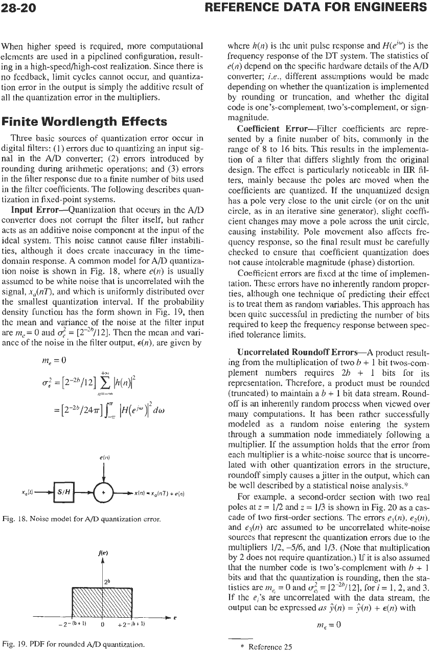
For example,

a

second-order section with two real

poles at

z

=

1/2 and

z

=

113 is shown

in

Fig.

20

as

a cas-

cade

of

two

first-order sections. The errors

el(n).

e2(n),

and

e&)

are assumed to be uncorrelated white-noise

sources that represent the quantization errors due to the

multipliers 1/2,

-5/6,

and 1/3. (Note that multiplication

by 2 does not require quantization.)

If

it is

also

assumed

that the number code is two's-complement with

b

+

1

bits and that the quantization is rounding, then the

sta-

tistics are

me,

=

0

and

crz

=

[2-Zb/12], fori

=

1,2, and 3.

If the

e,'s

are uncorrelated with

the

data stream, the

output can be expressed

as

j(n)

=

E(.)

+

~(n)

with

m,

=

0

*

Reference

25

DISCRETE-TIME SIGNAL PROCESSING

28-2

1

Fig.

20.

Second-order

and

n=O

11=0

where

h(n)

=

[(1/2)"

+

(1/3)"]u(n)

is the overall system

h,(n)

=

(1/3)'u(n)

is the unit pulse response of the

Furthermore, it is found that

d

=

[7.26/12]2-". If the

order of the sections

is

interchanged, a similar analysis

reveals that

d

=

[9.89/12]2-". This demonstrates that

the error accumulation in the output of a cascade filter

depends on the ordering of the sections, and that in

general there is a preferred ordering (the first in this

case).

This general approach to the analysis of arithmetic

quantization errors can be extended

to

higher-order fil-

ters realized in any configuration, provided the transfer

functions (unit pulse responses) from each noise

source to the filter output can be determined. Noise

analysis is particularly well suited for computer-aided

analysis routines that obtain the required transfer func-

tion as a step during a frequency-domain analysis.

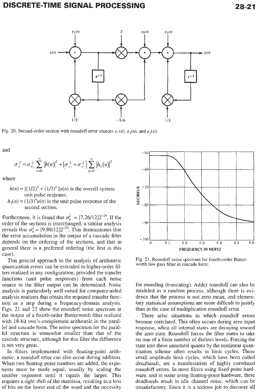
Figs. 21 and 22 show the roundoff noise spectrum at

the output of a fourth-order Butterworth filter realized

with 18-bit two's-complement arithmetic in the paral-

lel and cascade

form.

The noise spectrum for the paral-

lel structure is somewhat smaller than that of the

cascade structure, although for this filter the difference

is not very great.

In

filters implemented with floating-point arith-

metic, a roundoff error can also occur during addition.

When two floating-point numbers are added, the expo-

nents must be made equal, usually by scaling the

smaller exponent until it equals the larger. This

requires a right shift of the mantissa, resulting in a loss

of

bits on the lower end of the word and the necessity

unit pulse response,

second section.

0

01

02

03

04

05

06

FREQUENCY

IN

HERTZ

Fig.

21.

Roundoff

noise

spectrum for fourth-order Butter

worth

low-pass filter in cascade

form.

for rounding (truncating). Adder roundoff can also be

modeled as a random process, although there is evi-

dence that the process is not zero mean, and elemen-

tary

statistical assumptions are more difficult to justify

than in the case of multiplicative roundoff error.

There arise situations in which roundoff errors

become correlated. This often occurs during zero input

response, when

all

internal states are decaying toward

the zero state. Roundoff forces the filter states to take

on one of a finite number of distinct levels. Forcing the

state into these unnatural quanta by the nonlinear quan-

tization scheme often results in limit cycles. These

small amplitude limit cycles, which have been called

deadbands,

are a manifestation of highly correlated

roundoff errors.

In

most filters using fixed-point hard-

ware, and in some using floating-point hardware, these

deadbands result in idle channel noise, which can be

unsatisfactory. Since it is a tedious job

to

discover

all

Middleton W.M. (ed.) Reference Data for Engineers: Radio, Electronics, Computer and Communications

Подождите немного. Документ загружается.