Middleton W.M. (ed.) Reference Data for Engineers: Radio, Electronics, Computer and Communications
Подождите немного. Документ загружается.

15-10
REFERENCE
DATA
FOR ENGINEERS
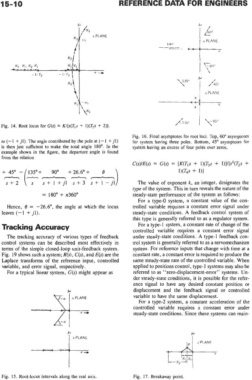
to
(-
1
t
jl).
The angle contributed by
the
pole
at
(-
1
+
jl)
is tRen just sufficient
to
make the total angle
180".
In
the
example shown in the figure,
the
departure angle is found
from
the
relation
=
180"
+
n360"
Hence,
0
=
-26.6",
the angle at which the locus
leaves (-1
+
jl).
Tracking Accuracy
The tracking accuracy of various types of feedback
control systems can be described most effectively in
terms of the simple closed-loop unit-feedback system.
Fig. 19 shows such a system;
R(s),
C(s),
and
E(s)
are the
Laplace transforms of the reference input, controlled
variable, and error signal, respectively.
For a typical linear system,
G(s)
might appear as
J[
s
PLANE
'[
s
PLANE
---t-
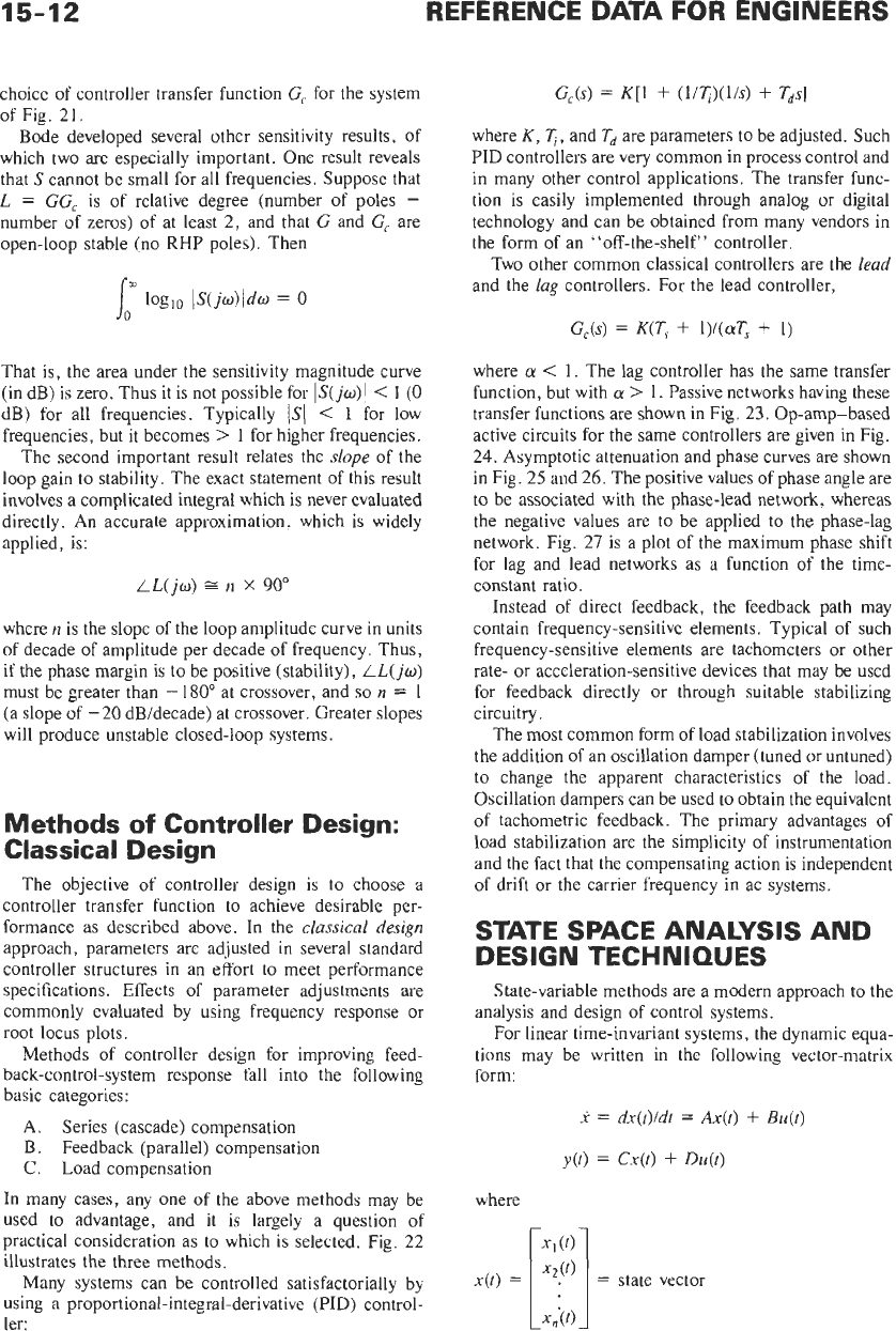
Fig.
15.
Root-locus
intervals along
the
real
axis.
s
PLANE
J
/
,L
135"
I\
\\-
450
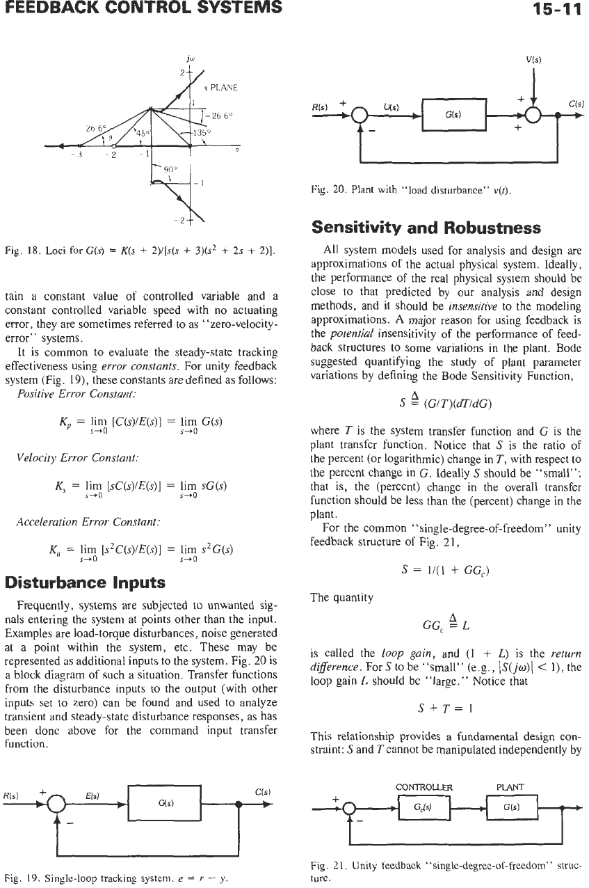
Fig.
16.
Final asymptotes for root loci. Top,
60"
asymptotes
for system having three poles. Bottom,
45"
asymptotes for
system having
an
excess of
four
poles
over
zeros.
The value of exponent
k,
an integer, designates the
type
of the system. This in turn reveals the nature of the
steady-state performance of the system as follows:
For a type-0 system, a constant value
of
the con-
trolled variable requires a constant error signal under
steady-state conditions.
A
feedback control system of
this type
is
generally referred to as a regulator system.
For
a
type-1 system, a constant rate of change
of
the
controlled variable requires a constant error signal
under steady-state conditions.
A
type- 1 feedback con-
trol system is generally referred to as a servomechanism
system. For reference inputs that change with time at a
constant rate, a constant error is required to produce the
same steady-state rate of the controlled variable. When
applied
to
positions control, type-1 systems may also be
referred to as "zero-displacement-error" systems. Un-
der steady-state conditions, it is possible for the refer-
ence signal to have any desired constant position or
displacement and the feedback signal or controlled
variable to have the same displacement.
For a type-2 system, a constant acceleration
of
the
controlled variable requires
a
constant error under
steady-state conditions. Since these systems can main-
Fig.
17.
Breakaway
point.
15-11
Fig.
18.
Loci
for
G(s)
=
K(s
+
2)/[s(s
+
3)(s2
+
2s
+
2)].
tain a constant value of controlled variable and a
constant controlled variable speed with no actuating
error, they are sometimes referred to as “zero-velocity-
error” systems.
It is common to evaluate the steady-state tracking
effectiveness using error constants.
For
unity feedback
system (Fig.
19),
these constants are defined as follows:
Positive Error Constant:
Kp
=
lim [C(s)/E(s)]
s-0
Velocity Error Constant:
Ks
=
lim [sC(s)/E(s)]
Acceleration Error Constant:
K,
=
lim
[s*C(s)/E(s)]
s-0
s-0
Disturbance Inputs
=
lim
G(s)
s-0
=
lim
sG(s)
S+O
=
lim
s2G(s)
s-0
Frequently, systems are subjected to unwanted sig-
nals entering the system at points other than the input.
Examples are load-torque disturbances, noise generated
at a point within the system, etc. These may be
represented as additional inputs to the system. Fig.
20
is
a block diagram
of
such a situation. Transfer functions
from the disturbance inputs to the output (with other
inputs set to zero) can be found and used to analyze
transient and steady-state disturbance responses, as has
been done above for the command input transfer
function.
Fig.
19.
Single-loop tracking system.
e
=
r
-
y.
Fig.
20.
Plant with
“load
disturbance”
v(f).
Sensitivity and Robustness
All system models used for analysis and design are
approximations of the actual physical system. Ideally,
the performance of the real physical system should be
close to that predicted by our analysis and design
methods, and it should be insensitive to the modeling
approximations. A major reason for using feedback is
the potential insensitivity
of
the performance of feed-
back structures to some variations in the plant. Bode
suggested quantifying the study of plant parameter
variations by defining the Bode Sensitivity Function,
S
=
(G/T)(dT/dG)
where
T
is
the system transfer function and
G
is the
plant transfer function. Notice that
S
is the ratio of
the percent (or logarithmic) change in
T,
with respect to
the percent change in
G.
Ideally
S
should be “small”;
that is, the (percent) change
in
the overall transfer
function should be less than the (percent) change in the
plant.
For the common “single-degree-of-freedom” unity
feedback structure of Fig.
21,
A
S
=
1/(1
+
GG,)
The quantity
A
GG,
=
L
is called the loop gain, and
(1
+
L)
is the return
dijference.
ForS to be “small” (e.g.,
\S(jo)(
<
I),
the
loop gain
L
should be “Iarge.” Notice that
S+T=1
This relationship provides a fundamental design
con-
straint:
S
and
T
cannot be manipulated independently by
CONTROLLER
PLANT
Fig.
21.
Unity feedback “single-degree-of-freedom”
struc-
ture.
15-12
REFERENCE DATA FOR ENGINEERS
choice of controller transfer function G, for the system
of Fig. 21.
Bode developed several other sensitivity results, of
which two are especially important. One result reveals
that
S
cannot be small for all frequencies. Suppose that
L
=
GG, is of relative degree (number of poles
-
number of zeros) of at least
2,
and that G and G, are
open-loop stable (no RHP poles). Then
That
is,
the area under the sensitivity magnitude curve
(in dB) is zero. Thus it is not possible for
IS(jw)l
<
1
(0
dB) for all frequencies. Typically
/SI
<
1
for low
frequencies, but it becomes
>
1
for higher frequencies.
The second important result relates the
slope
of the
loop gain to stability. The exact statement of this result
involves a complicated integral which is never evaluated
directly. An accurate approximation, which is widely
applied, is:
LL(jw)
n
x
90"
where
n
is the slope of the loop amplitude curve
in
units
of decade of amplitude per decade of frequency. Thus,
if the phase margin is
to
be positive (stability),
LL(
jo)
must be greater than
-
180"
at crossover, and
so
n
=
1
(a slope of
-20
dBidecade) at crossover. Greater slopes
will produce unstable closed-loop systems.
Methods
of
Controller Design:
Classical
Design
The objective of controller design is to choose a
controller transfer function to achieve desirable per-
formance as described above.
In
the
classical
design
approach, parameters are adjusted in several standard
controller structures in an effort to meet performance
specifications. Effects
of
parameter adjustments are
commonly evaluated by using frequency response or
root locus plots.
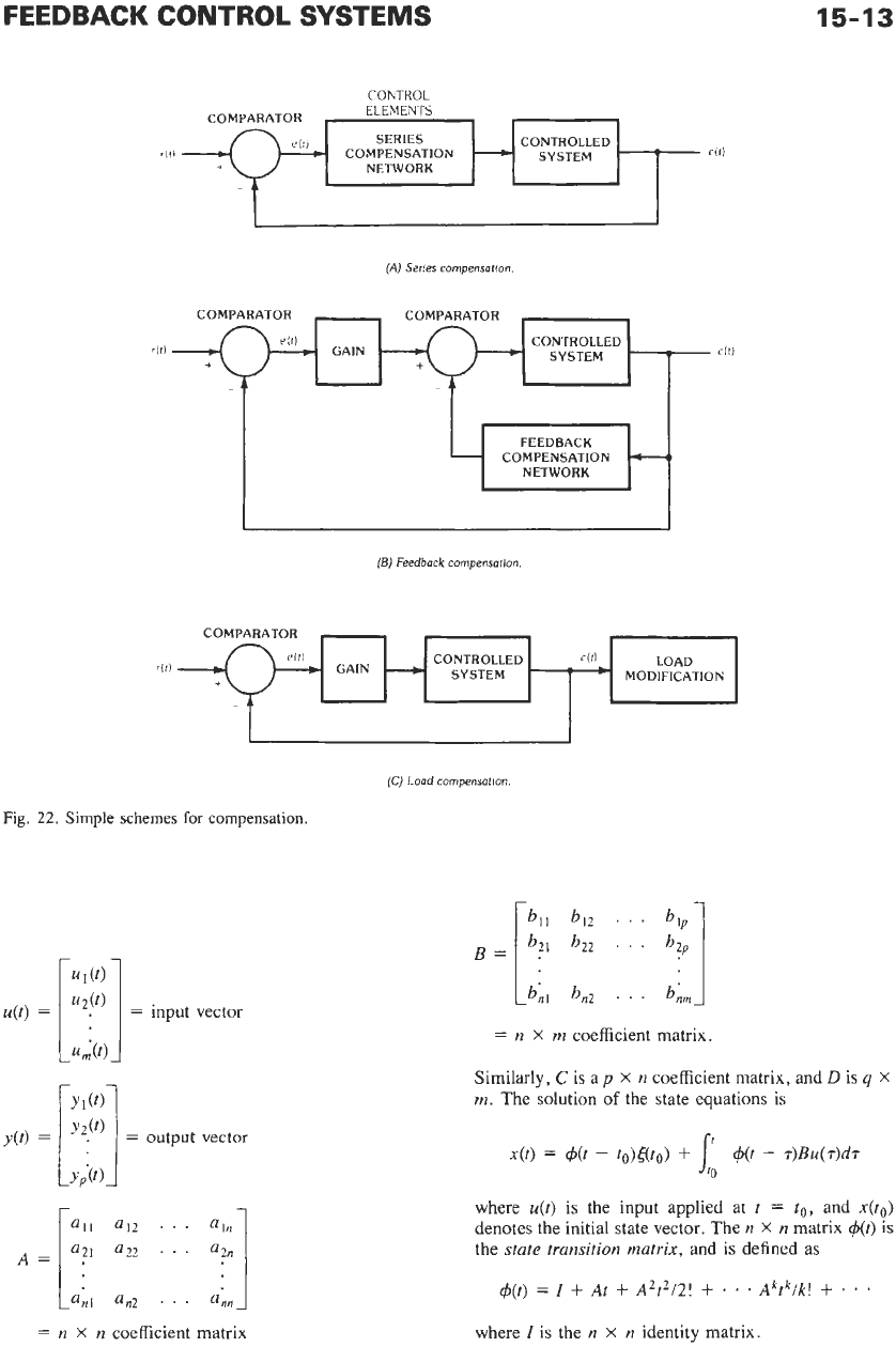
Methods of controller design for improving feed-
back-control-system response fall into the following
basic categories:
A.
Series (cascade) compensation
B
.
Feedback (parallel) compensation
C.
Load compensation
In
many cases, any one
of
the above methods may be
used to advantage, and it is largely
a
question of
practical consideration as to which is selected. Fig. 22
illustrates the three methods.
Many systems can be controlled satisfactorially by
using a proportional-integral-derivative (PID) control-
ler:
GJs)
=
K[1
+
(l/T)(l/s)
+
TdSl
where
K,
q,
and
Td
are parameters
to
be adjusted. Such
PID controllers are very common in process control and
in
many other control applications. The transfer func-
tion is easily implemented through analog or digital
technology and can be obtained from many vendors in
the form of an "off-the-shelf" controller.
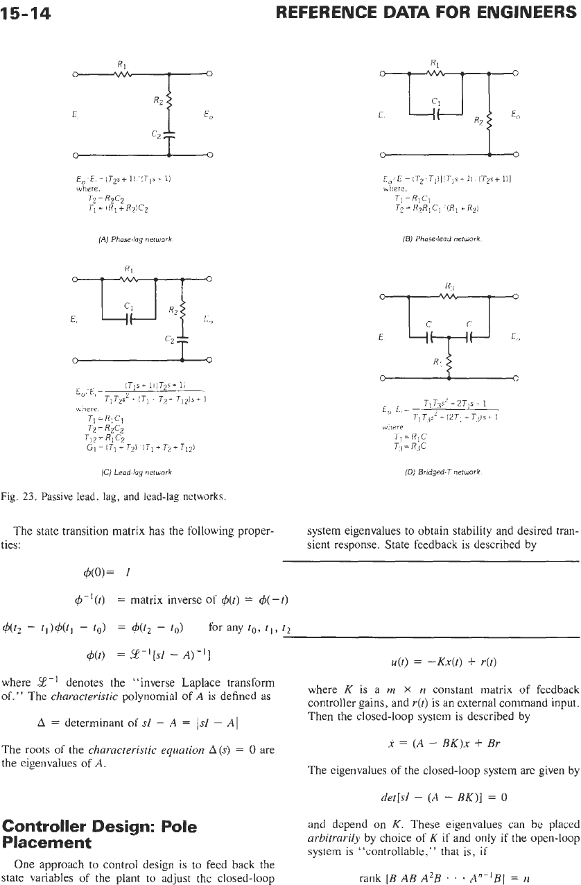
Two other common classical controllers are the
lead
and the
lag
controllers. For the lead controller,
G,(s)
=
K(T,
+
l)/(cuT,
+
1)
where
a
<
1.
The lag controller has the same transfer
function, but with
a
>
1. Passive networks having these
transfer functions are shown in Fig.
23.
Op-amp-based
active circuits for the same controllers are given in Fig.
24.
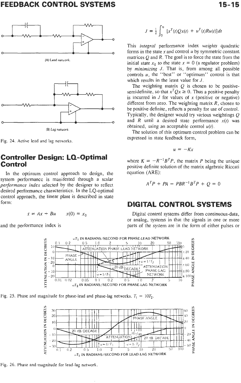
Asymptotic attenuation and phase curves are shown
in
Fig. 25 and
26.
The positive values of phase angle are
to be associated with the phase-lead network, whereas
the negative values are
to
be applied to the phase-lag
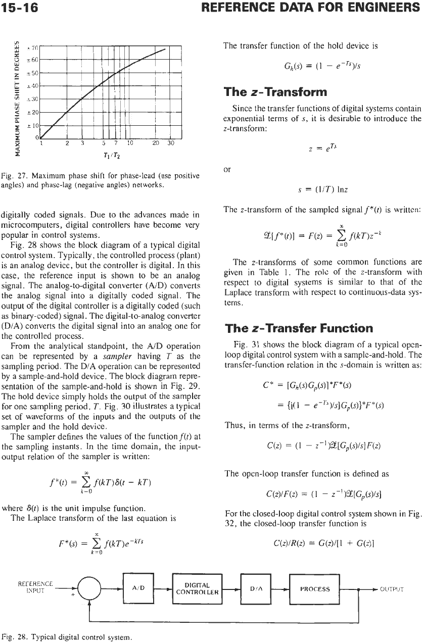
network. Fig.
27
is a plot of the maximum phase shift
for lag and lead networks as a function of the time-
constant ratio.
Instead of direct feedback, the feedback path may
contain frequency-sensitive elements. Typical of such
frequency-sensitive elements are tachometers or other
rate- or acceleration-sensitive devices that may be used
for feedback directly or through suitable stabilizing
circuitry.
The most common form of load stabilization involves
the addition of an oscillation damper (tuned or untuned)
to change the apparent characteristics of the load.
Oscillation dampers can be used to obtain the equivalent
of tachometric feedback. The primary advantages of
load stabilization are the simplicity of instrumentation
and the fact that the compensating action is independent
of drift
or
the carrier frequency
in
ac systems.
STATE §PACE ANALYSIS AND
DESIGN TECHNIQUES
State-variable methods are a modern approach to the
analysis and design of control systems.
For linear time-invariant systems, the dynamic equa-
tions may be written in the following vector-matrix
form:
where
x(t)
=
FEEDBACK CONTROL
SYSTEMS
SERIES
NETWORK
rlil
COMPENSATION
15-13
CONTROLLED
C(l)
-
SYSTEM
ritl
GAIN
(A)
Series compensation,
clti
CONTROLLED
SYSTEM
-
-
FEEDBACK
NETWORK
-
COMPENSATION
-1
(E)
Feedback compensation
ri0
CONTROLLED
C(t1
LOAD
SYSTEM
*
MODIFICATION
GAIN
-
(C)
Load compensation,
Fig.
22.
Simple
schemes
for
compensation.
=
n
x
m
coefficient matrix.
Similarly,
C
is ap
X
n
coefficient matrix, and
D
is
q
X
m.
The solution
of
the state equations is
x(t)
=
d(t
-
to)&o)
-t
1:
d(t
-
T)Bu(T)d7
where
u(t)
is the input applied at
t
=
to,
and
x(t0)
denotes the initial state vector. The
n
X
n
matrix
&t)
is
the
state
transition matrix,
and is defined as
+(t)
=
I
+
At
+
A2t2/2!
+
*
. .
Aktk/k!
+
. .
.
where
I
is the
n
X
n
identity matrix.
=
n
x
n
coefficient matrix
15-14
REFERENCE
DATA
FOR
ENGINEERS
E,'E,=
(Tqsf
l).'(Tis+
1)
where.
(A)
Phose-lag
network.
O
0
(C)
Lead-lag
network
Fig.
23.
Passive
lead,
lag,
and
lead-lag networks.
(B) Phase-lead
network
TI
JJS'
+
2
Jls
-
1
E,
E,=
T1T~sL+(2J:+J~ls+1
where
7'1
=R1C
r.+
=
R,~C
(D)
Bridged-T
network.
The state transition matrix has the following proper- system eigenvalues to obtain stability and desired tran-
sient response. State feedback is described by
ties:
where
2-l
denotes the "inverse Laplace transform
of." The
characteristic
polynomial
of
A
is
defined
as
where
K
is a
rn
X
n
constant matrix
of
feedback
controller gains, and
r(t)
is
an external command input.
Then the closed-loop system is described by
A
=
determinant of
sf
-
'4
=
Isf
-
AI
The roots of the
characteristic equation
A(s)
=
0
are
the eigenvalues of
A.
x
(A
-
BK)x
+
Br
The eigenvalues
of
the closed-loop system are given by
det[sI
-
(A
-
BK)]
=
0
Controller Design: Pole
Placement
One approach to control design is to feed back the
state variables of the plant to adjust the closed-loop
rank
[B
AB
A2B
.
. .
A"-'B]
=
n
and depend
on
K.
These eigenvalues can be placed
arbitrarily
by choice of
K
if and only if the open-loop
svstem is "controllable." that is. if
FEEDBACK CONTROL SYSTEMS
15-15
I/
0
vvb
0
(A)
Lead network.
*
fBj
Lag network.
Fig.
24.
Active lead and lag networks
Controller Design:
LQ-Optimal
Control
In the optimum control approach to design, the
system performance is manifested through a scalar
performance index
selected by the designer to reflect
desired performance characteristics. In the LQ-optimal
control approach, the linear plant is described in state
form:
and the performance index is
d
=
[xT(t)Qx(t)
+
uT(t)Ru(t)]dt
This
integral
performance index
weights
quadratic
forms in the state
x
and control
u
by symmetric constant
matrices
Q
and
R.
The goal is to force the state from the
initial state
xo
to the state
x
=
0
(a regulator problem)
by
minimizing
J.
That
is,
from among all possible
controls
u,
the “best” or “optimum” control is that
which results in the least value for
J.
The weighting matrix
Q
is
chosen to be positive-
semidefinite,
so
that
xTQx
2
0.
Thus a positive penalty
is incurred in
J
for values
of
x
(positive or negative)
different from zero. The weighting matrix
R,
chosen to
be positive definite, reflects a penalty for use of control.
Typically, the designer would
try
various weightings Q
and
R
until a desired state performance
x(t)
was
obtained, using an acceptable control
u(t).
The solution of this optimum control problem can be
expressed
in
state feedback form,
u
=
-Kx
where
K
=
-R-’BTP,
the matrix
P
being the unique
positive definite solution
of
the matrix algebraic Riccati
equation (ARE):
ATP
i-
PA
-
PBR-‘BTP
+
Q
=
0
DIGITAL CONTROL SYSTEMS
Digital control systems differ from continuous-data,
or analog, systems in that the signals in one or more
parts of the system are in the form of either pulses or
Fig.
25.
Phase and
*rl
IN
RADIANS/SECOND
FOR
PHASE-LEAD
NETWORK
m
’
01
02 05
10
2
5
10
20
50
100
y
0%
5-10
f40
5
2-20
30
$-lo
t80
2
2-20
f
‘00%
L
UT2
IN RADlANS/SECOND FOR PHASE-LAG NETWORK
2
g
10
Yo
I20
2
Lil
260
d
W
001
002 005 01
02
05
10
2
5
IO
d
4
magnitude
for
phase-lead and phase-lag networks.
TI
=
lor2.
J)
‘n
G:
30 60
y
20
40
g
20
:
Y
0
10
z
z
0
5
e
-
10
5
-20
-40
2
5
(11
02
05
10
2
5 10 20
a
-20
0
z
-
60
2
ti
-
30
50
100
E
wT1
IN RADIANS/SECOND FOR LEAD-LAG NETWORK
Fig.
26.
Phase and magnitude for lead-lag network.
15-16
A/D
-c
REFERENCE
INPUT
REFERENCE
DATA
FOR ENGINEERS
D!A
-
PROCESS
2
OUTPUT
DIGITAL
CONTROLLER
-
Fig.
27.
Maximum phase
shift
for phase-lead
(use
positive
angles)
and
phase-lag (negative angles) networks.
digitally coded signals. Due to the advances made in
microcomputers, digital controllers have become very
popular in control systems.
Fig.
28
shows the block diagram of a typical digital
control system. Typically, the controlled process (plant)
is an analog device, but the controller is digital.
In
this
case, the reference input is shown to be an analog
signal. The analog-to-digital converter
(AID)
converts
the analog signal into a digitally coded signal. The
output of the digital controller
is
a digitally coded (such
as binary-coded) signal. The digital-to-analog converter
(D/A) converts the digital signal into an analog one for
the controlled process.
From the analytical standpoint, the AID operation
can be represented by a
sampler
having
T
as the
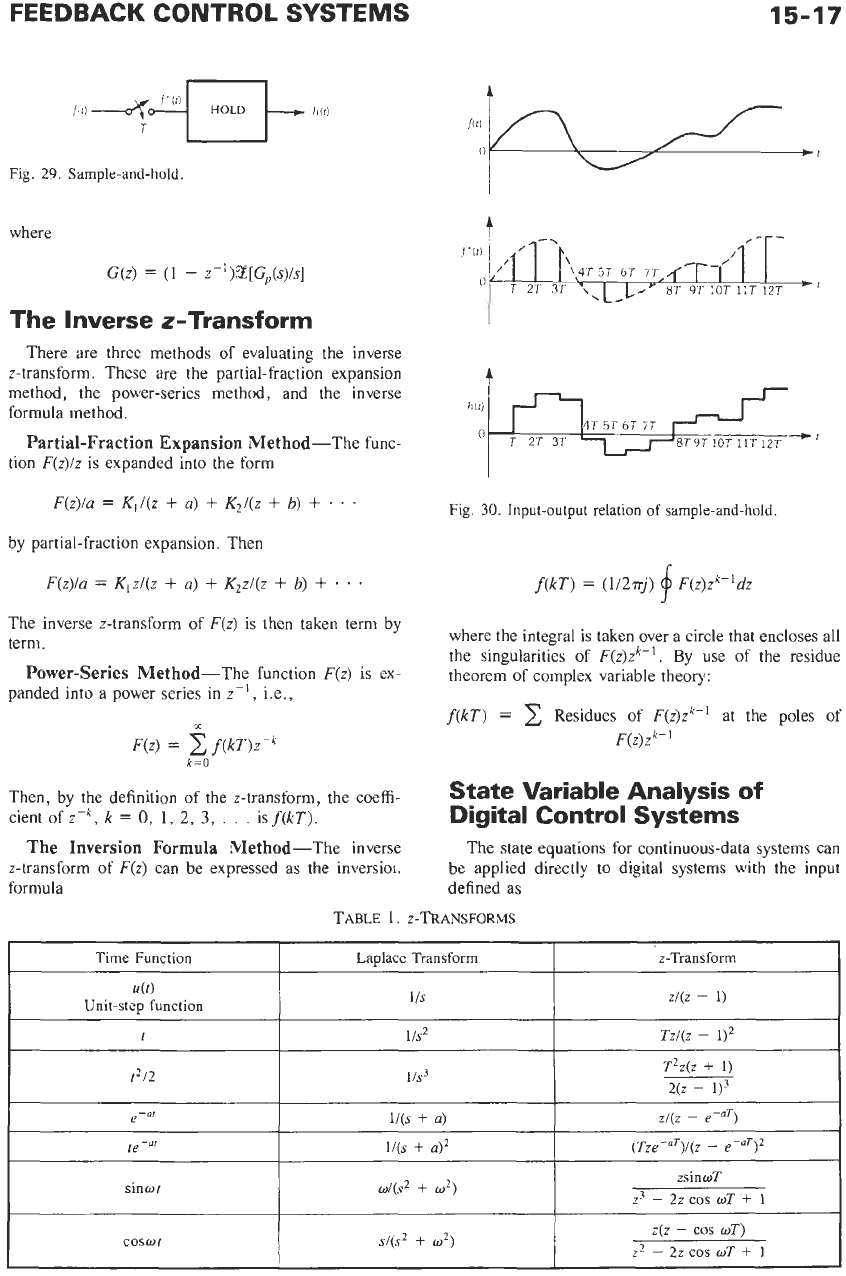
sampling period. The D/A operation can be represented
by a sample-and-hold device. The block diagram repre-
sentation of the sample-and-hold is shown in Fig.
29.
The hold device simply holds the output of the sampler
for one sampling period,
T.
Fig.
30
illustrates a typical
set of waveforms of the inputs and the outputs of the
sampler and the hold device.
The sampler defines the values of the functionf(t) at
the sampling instants.
In
the time domain, the input-
output relation of the sampler is written:
P
f*(t)
=
c,
f(kT)S(t
-
kT)
k=O
where
S(t)
is the unit impulse function.
The Laplace transform
of
the last equation is
The transfer function of the hold device is
G,(s)
=
(1
-
CTS)/s
The
z-Transform
Since the transfer functions of digital systems contain
exponential terms of
s,
it is desirable to introduce the
z-transform:
=
eTs
or
s
=
(UT)
lnz
The z-transform of the sampled signal
f*(t)
is written:
m
%[f*(t)J
=
F(z)
=
f(kT)z-k
k=O
The z-transforms of some common functions are
given in Table 1. The role of the z-transform with
respect to digital systems is similar to that of the
Laplace transform with respect to continuous-data sys-
tems.
The
z-Transfer Function
Fig. 31 shows the block diagram
of
a typical open-
loop digital control system with a sample-and-hold. The
transfer-function relation in the s-domain is written as:
C*
=
[G~(s)G,(s)]*F*(s)
=
{[(l
-
e-Ts)/s]G,(s)}*F*(s)
Thus, in terms of the z-transform,
C(z)
=
(1
-
z-’)%.[G,(s)/s]F(z)
The open-loop transfer function is defined as
C(z)/F(z)
=
(1
-
~-~)%[G,(s)/s]
For the closed-loop digital control system shown in Fig.
32,
the closed-loop transfer function is
C(z)IR(z)
=
G(z)/[l
+
G(z)]
L
J
Fig.
28.
Typical
digital
control system.
FEEDBACK
CONTROL
SYSTEMS
Time Function
u
(t)
Unit-step function
15-17
Laplace Transform z-Transform
z/(z
-
1)
1
is
Fig.
29.
Sample-and-hold
e-llt
where
l/(s
+
a)
z/(z
-
e-aT)
G(z)
=
(1
-
z-')Z[GP(~)/s]
The
Inverse z-Transform
te-"'
sinot
There are three methods of evaluating the inverse
z-transform. These are the partial-fraction expansion
method, the power-series method, and the inverse
formula method.
Partial-Fraction
Expansion
Method-The func-
tion
F(z)/z
is expanded into the form
F(z)/a
=
K,/(z
+
a)
+
K2/(z
+
b)
+
.
.
*
by partial-fraction expansion. Then
I/(S
+
a)'
d(S2
+
02)
(Tze-uT)/(z
-
e-aT)2
zsinwT
z3
-
22
cos
wT
+
1
F(z)/a
=
K~Z/'(Z
+
a)
+
K>z/(z
+
b)
+
. .
The inverse z-transform of F(z) is then taken term by
term.
Power-Series Method-The function
F(z)
is ex-
panded into a power series in
z-',
i.e.,
3c
F(z)
=
2
f(k7,)z-k
k=O
Then, by the definition of the z-transform, the coeffi-
cient of
z-~,
k
=
0,
I,
2,
3,
.
.
.
isf(kT).
The
Inversion
Formula
Method-The inverse
z-transform of
F(z)
can be expressed as the inversioi,
formula
c
4
Fig.
30.
Input-output relation of sample-and-hold.
f(kT)
=
(11271-J)
F(z)zk-'dz
i
where the integral is taken over a circle that encloses all
the singularities of
F(z)zk-'.
By use of the residue
theorem
of
complex variable theory:
f(kT)
=
2
Residues
of
F(z)zk-' at the poles of
F(z)zk-'
State Variable Analysis
of
Digital Control Systems
The state equations for continuous-data systems can
be applied directly to digital systems with the input
defined as
TABLE
1.
2-TRANSFORMS
t
I
lis2
I
Tz/(z
-
1)*
COSOt
s/(s2
+
02)
z(z
-
cos
UT)
22
-
22
cos
wT
+
1

15-18
REFERENCE DATA
FOR
ENGINEERS
Illti
HOLD
Clll
Fig.
3
1.
Open-loop
digital
control
system
u(t)
=
u(kT)
kT
5
t
<
(k
+
l)T
due to the action of the sample-and-hold. Thus, the
state equations of an nth-order digital system are written
as
dx(t)ldt
=
h(t)
+
Bu(kT)
kT
5
t
<
(k
+
l)T
The solution of the state equation, the state transition
equation, is
x(t)
=
+(t
-
kT)x(kT)
+
+(t
-
7)BdT
*
u(kT)
Let
Then,
x(t)
=
fit
-
,w)x(k~)
+
e(t
-
k~)u(kr)
To
describe the state variables only at the sampling
instants, let
t
=
(k
+
1)T.
The last equation becomes
x[(k
+
I)T]
=
+((T)x(kT)
+
B(T)u(kT)
which is the form of a vector-matrix difference equation
with constant coefficients. The solution of this differ-
ence equation is
and
A2T2
A3T3
2!
3!
+(TI
=
eAT
=
I
+
AT
+
-
+-+...
Stability
of
Linear
Time- Invariant Digital Systems
The stability-analysis methods devised for linear
continuous-data systems can all be extended to the
stability study
of
digital systems. Since the z-transfor-
mation
z
=
e''
maps the imaginary axis in the s-plane
onto the unit circle,
/z/
=
I,
in the z-plane, the stability
criterion
of
linear time-invariant digital systems is that
all the roots of the characteristic equation must be found
inside the unit circle in the z-plane.
The stability of the digital control system shown
in
Fig.
32
depends on the location
of
the poles of the
closed-loop transfer function
C(z)IR(z)
=
G(z)/[l
+
G(z)l
or of the zeros of
1
+
G(z)
in the complex z-plane.
the characteristic equation, which can be written as
The zeros of
1
+
G(z)
are also known as the roots
of
F(z)
=
u,z"
+
u,-lz"-l
+
'
'
.
+
a2z2
+
a0
=
0
where all the coefficients are real.
The tabulation in Chart 1, known as the
Jury
Table,
can be formed to check the necessary and sufficient
conditions for the roots
of
the characteristic equations
to be inside the unit circle.
The conclusion are:
Number of
positive
calculated elements in the first
column,
(bo,
co,
.
.
.
,
po,
qo,
ro)
=
number of
roots inside the unit circle.
Number of
negative
calculated elements in the first
column,
(bo,
eo,
. .
.
,
po,
qo,
yo)
=
number of
roots outside the unit circle.
~q-H-1
HOLD
till1
G,,W
c(Il
Fig.
32.
Closed-loop digital control system.
FEEDBACK
CONTROL
SYSTEMS
15-19
CHART
1.
CHART
FOR
CHECKING CONDITIONS
FOR
ROOTS
OF
CHARACTERISTIC EQUATIONS
TO
BE
INSIDE
UNIT
CIRCLE
...
Po PI P? kp
=
P21PO
P2kp P
I
lk,
90
41
k,
=
4140
4lko
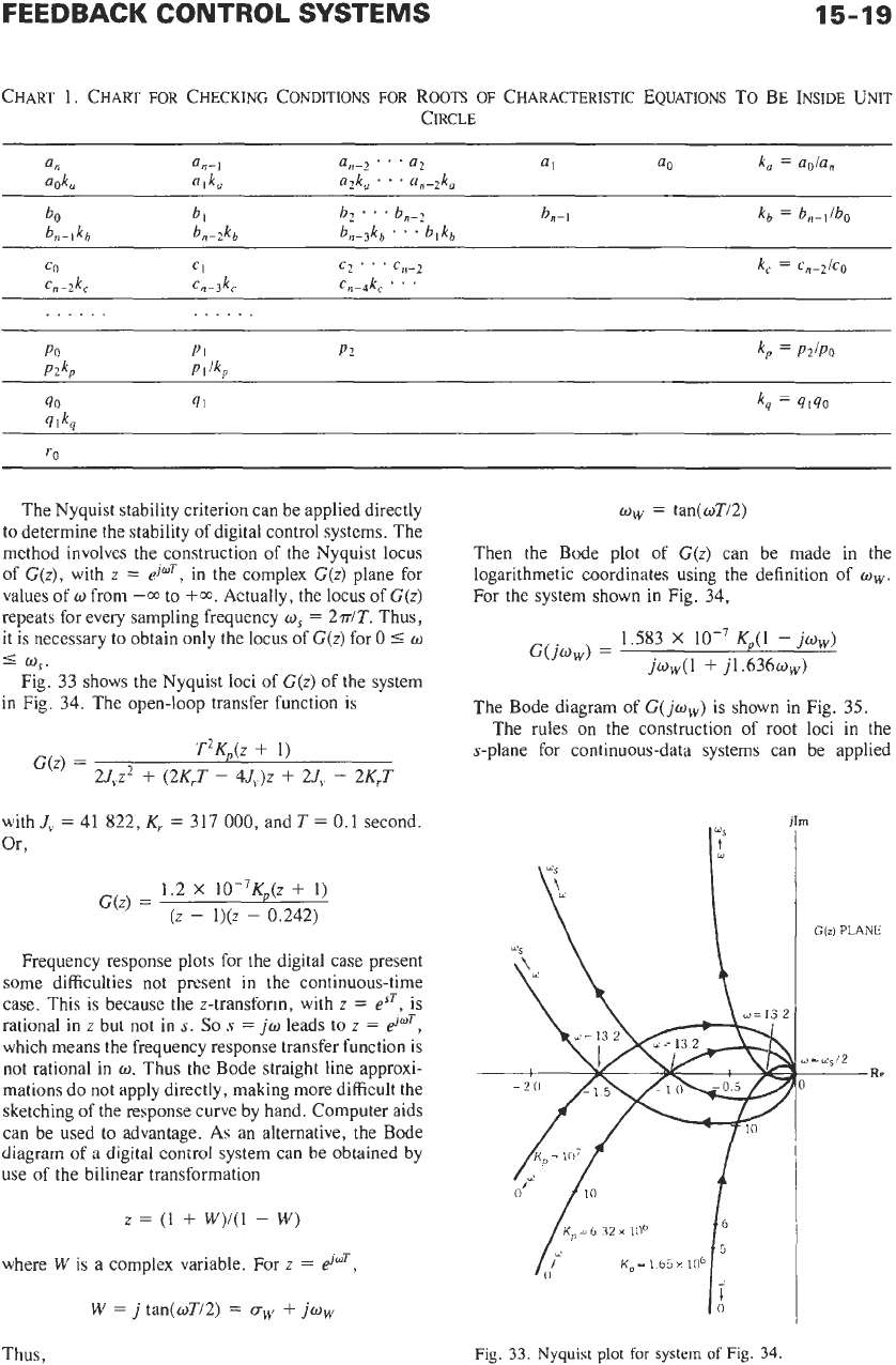
The Nyquist stability criterion can be applied directly
to determine the stability of digital control systems. The
method involves the construction of the Nyquist locus
of G(z), with
z
=
ejmT,
in the complex G(z) plane for
values of
w
from
--oo
to
+a;.
Actually, the locus of G(z)
repeats for every sampling frequency
o,
=
2dT. Thus,
it is necessary to obtain only the locus of G(z) for
0
5
w
5
w,.
Fig. 33 shows the Nyquist loci of G(z) of the system
in Fig. 34. The open-loop transfer function is
T2K,(z
+
1)
2J,z2
+
(2KrT
-
4J,)z
+
U,
-
2K,T
G(z)
=
with
J,
=
41
822,
K,
=
317
000,
and
T
=
0.1
second.
Or,
1.2
x
10-7~~~
+
1)
G(z)
=
(z
-
l)(z
-
0.242)
Frequency response plots for the digital case present
some difficulties not present in the continuous-time
case. This is because the z-transform, with
z
=
esT?
is
rational in
z
but not
in
s.
So
s
=
jw
leads to
z
=
eJmT,
which means the frequency response transfer function is
not rational in
w.
Thus the Bode straight line approxi-
mations do not apply directly, making more difficult the
sketching of the response curve by hand. Computer aids
can be used to advantage.
As
an alternative, the Bode
diagram
of
a digital control system can be obtained by
use of the bilinear transformation
z
=
(1
+
W)/(l
-
W)
where
W
is a complex variable. For
z
=
eloT,
W
=
j
tan(oTi2)
=
uw
+
jw,
ww
=
tan(wTi2)
Then the Bode plot
of
G(z)
can be made in the
logarithmetic coordinates using the definition of
ww
.
For the system shown in Fig. 34,
1.583
X
KJ1
-
jw,)
G(jww)
=
jww(l
+
j1.636~~)
The Bode diagram
of
G(jw,) is shown in Fig. 35.
The rules on the construction of root loci in the
s-plane for continuous-data systems can be applied
I
Giz)
PLANE
>=42
Re
Thus,
Fig.
33.
Nyquist
plot
for
system
of
Fig.
34.