Raven P.H., Johnson G.B., Mason K.A. Biology (Ninth Edition)
Подождите немного. Документ загружается.

Apago PDF Enhancer
;2;10
Change in Clutch Size
Clutch Size Following Year
:1:2
7
6
5
8 10 12 14 0 2 4 6
Clutch Size
17.5
18.0
18.5
19.0
19.5
Nestling Size (g)
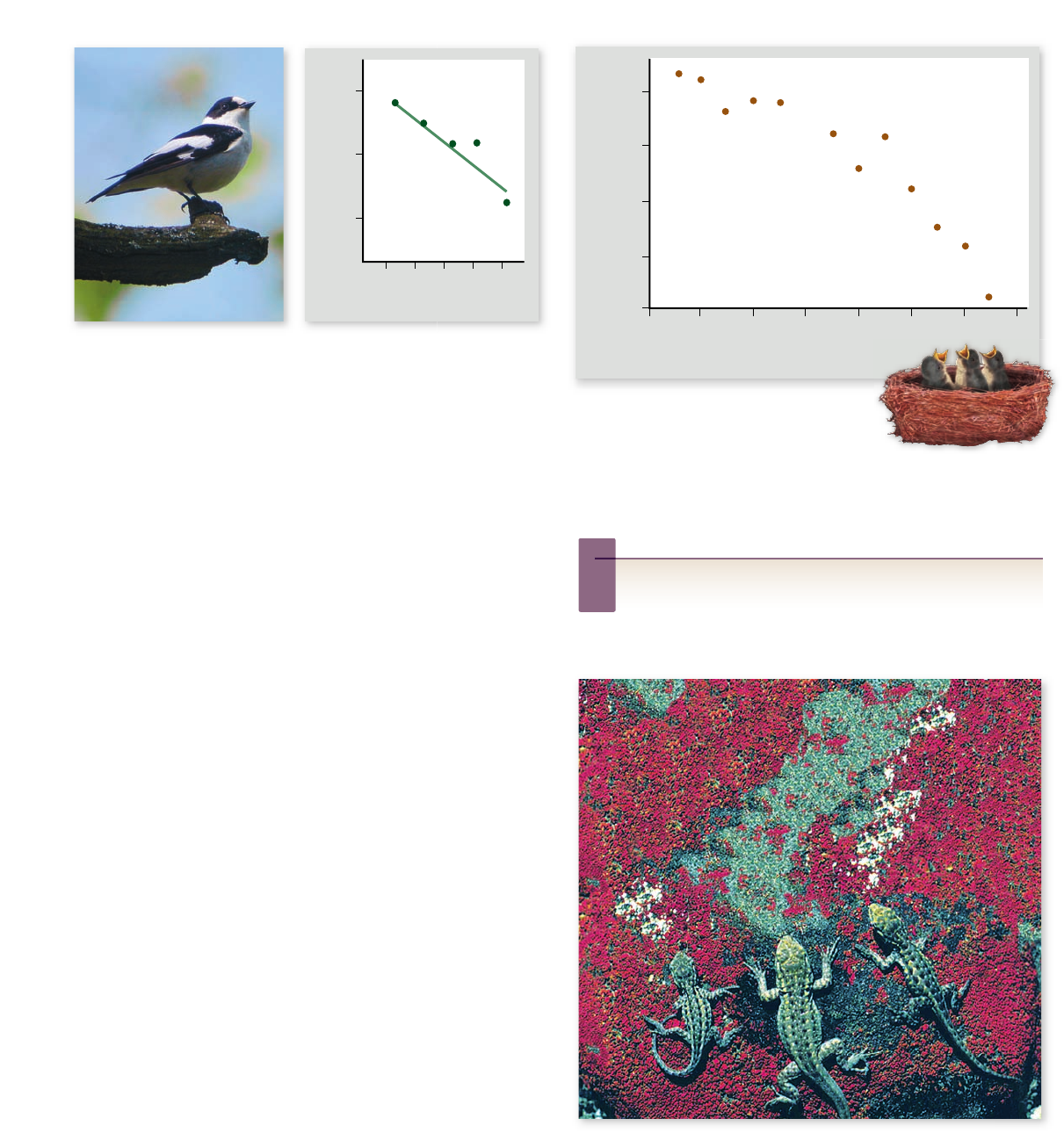
Figure 56.14
The relationship
between clutch size and o spring size.
In great tits (Parus major), the size of the
nestlings is inversely related to the number of eggs
laid. The more mouths they have to feed, the less the parents can
provide to any one nestling.
Inquiry question
?
Would natural selection favor producing many small young or
a few large ones?
Figure 56.13
Reproductive events per lifetime.
Adding
eggs to nests of collared ycatchers (Ficedula albicollis), which
increases the reproductive efforts of the female rearing the young,
decreases clutch size the following year; removing eggs from the
nest increases the next year’s clutch size. This experiment
demonstrates the trade-off between current reproductive effort
and future reproductive success.
Natural selection favors the life history that maximizes
lifetime reproductive success. When the cost of reproduction is
low, individuals should produce as many offspring as possible
because there is little cost. Low costs of reproduction may oc-
cur when resources are abundant and may also be relatively low
when overall mortality rates are high. In the latter case, indi-
viduals may be unlikely to survive to the next breeding season
anyway, so the incremental effect of increased reproductive ef-
forts may have little effect on future survival.
Alternatively, when costs of reproduction are high, life-
time reproductive success may be maximized by deferring or
minimizing current reproduction to enhance growth and sur-
vival rates. This situation may occur when costs of reproduc-
tion significantly affect the ability of an individual to survive or
decrease the number of offspring that can be produced in
the future.
A trade-o exists between number
of o spring and investment per o spring
In terms of natural selection, the number of offspring pro-
duced is not as important as how many of those offspring
themselves survive to reproduce. Assuming that the amount of
energy to be invested in offspring is limited, a balance must be
reached between the number of offspring produced and the
size of each offspring (figure 56.14) . This trade-off has been
experimentally demonstrated in the side-blotched lizard,
which normally lays between four and five eggs at a time.
When some of the eggs are removed surgically early in the
reproductive cycle, the female lizard produces only one to
three eggs, but supplies each of these eggs with greater
amounts of yolk, producing eggs and, subsequently, hatchlings
that are much larger than normal (figure 56.15) . Alternatively,
by removing yolk from eggs, scientists have demonstrated
that smaller young would be produced.
Figure 56.15
Variation in the size of baby side-
blotched lizards (Uta stansburiana) produced by
experimental manipulations. In clutches in which some
developing eggs were surgically removed, the remaining offspring were
larger (center) than lizards produced in control clutches in which all the
eggs were allowed to develop (right). In experiments in which some of
the yolk was removed from the eggs, smaller lizards hatched (left).
117 2
part
VIII
Ecology and Behavior
rav32223_ch56_1162-1184.indd 1172rav32223_ch56_1162-1184.indd 1172 11/20/09 1:47:04 PM11/20/09 1:47:04 PM

Apago PDF Enhancer
In the side-blotched lizard and many other species, the
size of offspring is critical—larger offspring have a greater
chance of survival. Producing many offspring with little
chance of survival might not be the best strategy, but pro-
ducing only a single, extraordinarily robust offspring also
would not maximize the number of surviving offspring.
Rather, an intermediate situation, in which several fairly
large offspring are produced, should maximize the number
of surviving offspring.
Reproductive events per lifetime
represent an additional trade-o
The trade-off between age and fecundity plays a key role in
many life histories. Annual plants and most insects focus all
their reproductive resources on a single large event and then
die. This life history adaptation is called semelparity. Organ-
isms that produce offspring several times over many seasons
exhibit a life history adaptation called iteroparity.
Species that reproduce yearly must avoid overtaxing
themselves in any one reproductive episode so that they will
be able to survive and reproduce in the future. Semelparity,
or “big bang” reproduction, is usually found in short-lived
species that have a low probability of staying alive between
broods, such as plants growing in harsh climates. Semelpar-
ity is also favored when fecundity entails large reproductive
cost, exemplified by Pacific salmon migrating upriver to
their spawning grounds. In these species, rather than invest-
ing some resources in an unlikely bid to survive until the
next breeding season, individuals put all their resources into
one reproductive event.
Age at rst reproduction
correlates with life span
Among mammals and many other animals, longer-lived species
put off reproduction longer than short-lived species, relative to
expected life span. The advantage of delayed reproduction is
that juveniles gain experience before expending the high costs
of reproduction. In long-lived animals, this advantage out-
weighs the energy that is invested in survival and growth rather
than reproduction.
In shorter-lived animals, on the other hand, time is of the
essence; thus, quick reproduction is more critical than juvenile
training, and reproduction tends to occur earlier.
Learning Outcomes Review 56.4
Life history adaptations involve many trade-off s between reproductive
cost and investment in survival. These trade-off s take a variety of forms,
from laying fewer than the maximum possible number of eggs to putting
all energy into a single bout of reproduction. Natural selection favors
maximizing reproductive success, but number of off spring produced must be
tempered by available resources.
■ How might the life histories of two species differ if one
was subject to high levels of predation and the other
had few predators?
56.5
Environmental Limits
to Population Growth
Learning Outcomes
Explain exponential growth.1.
Discuss why populations cannot grow exponentially forever.2.
Define carrying capacity.3.
Populations often remain at a relatively constant size, regard-
less of how many offspring are born. As you saw in chapter 1,
Darwin based his theory of natural selection partly on this
seeming contradiction. Natural selection occurs because of
checks on reproduction, with some individuals producing fewer
surviving offspring than others. To understand populations, we
must consider how they grow and what factors in nature limit
population growth.
The exponential growth model applies
to populations with no growth limits
The rate of population increase, r, is defined as the difference be-
tween the birth rate, b, and the death rate, d, corrected for move-
ment of individuals in or out of the population (e, rate of movement
out of the area; i, rate of movement into the area). Thus,
r = (b – d ) + (i – e)
Movements of individuals can have a major influence on
population growth rates. For example, the increase in human
population in the United States during the closing decades of
the 20th century was mostly due to immigration.
The simplest model of population growth assumes that
a population grows without limits at its maximal rate and also
that rates of immigration and emigration are equal. This rate,
called the biotic potential, is the rate at which a population
of a given species increases when no limits are placed on its
rate of growth. In mathematical terms, this is defined by the
following formula:
dN
dt
= r
i
N
where N is the number of individuals in the population, dN/dt
is the rate of change in its numbers over time, and r
i
is the in-
trinsic rate of natural increase for that population—its innate
capacity for growth.
The biotic potential of any population is exponential (red
line in figure 56.16). Even when the rate of increase remains
constant, the actual number of individuals accelerates rapidly as
the size of the population grows. The result of unchecked expo-
nential growth is a population explosion.
A single pair of houseflies, laying 120 eggs per genera-
tion, could produce more than 5 trillion descendants in a year.
In 10 years, their descendants would form a swarm more than
2 m thick over the entire surface of the Earth! In practice, such
patterns of unrestrained growth prevail only for short periods,
usually when an organism reaches a new habitat with abundant
chapter
56
Ecology of Individuals and Populations
117 3www.ravenbiology.com
rav32223_ch56_1162-1184.indd 1173rav32223_ch56_1162-1184.indd 1173 11/20/09 1:47:06 PM11/20/09 1:47:06 PM
Apago PDF Enhancer
Positive
Growth
Rate
Negative
Growth
Rate
N = K
Below K Carrying
Capacity (K)
Above K
Population Size (N)
Population Growth Rate (dN/dt)
0
0 5 10
Number of Generations (t)
Population Size (N)
15
1250
1000
750
= 1.0 N
dN
dt
500
250
0
= 1.0 N
Carrying
capacity
dN
dt
1000 – N
1000
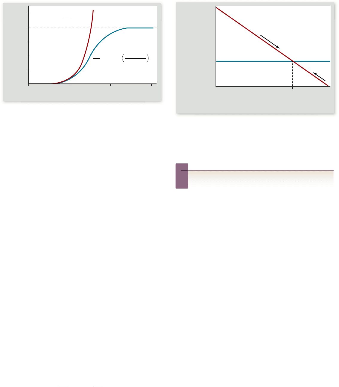
Figure 56.17
Relationship between population growth
rate and population size.
Populations far from the carrying
capacity (K) have high growth rates—positive if the population is
below K, and negative if it is above K. As the population approaches
K, growth rates approach zero.
Inquiry question
?
Why does the growth rate converge on zero?
Figure 56.16
Two models of population growth.
The
red line illustrates the exponential growth model for a population
with an r of 1.0. The blue line illustrates the logistic growth model
in a population with r = 1.0 and K = 1000 individuals. At rst,
logistic growth accelerates exponentially; then, as resources become
limited, the death rate increases and growth slows. Growth ceases
when the death rate equals the birth rate. The carrying capacity (K)
ultimately depends on the resources available in the environment.
resources. Natural examples of such short period of unre-
strained growth include dandelions arriving in the fields, lawns,
and meadows of North America from Europe for the first time;
algae colonizing a newly formed pond; or cats introduced to an
island with many birds, but previously lacking predators.
Carrying capacity
No matter how rapidly populations grow, they eventually reach
a limit imposed by shortages of important environmental fac-
tors, such as space, light, water, or nutrients. A population ulti-
mately may stabilize at a certain size, called the carrying
capacity of the particular place where it lives. The carrying ca-
pacity, symbolized by K, is the maximum number of individuals
that the environment can support.
The logistic growth model applies to
populations that approach their
carrying capacity
As a population approaches its carrying capacity, its rate of
growth slows greatly, because fewer resources remain for
each new individual to use. The growth curve of such a popu-
lation, which is always limited by one or more factors in the
environment, can be approximated by the following logistic
growth equation:
dN
dt
= rN
(
K – N
K
)
In this model of population growth, the growth rate of the
population (dN/dt) is equal to its intrinsic rate of natural increase
(r multiplied by N, the number of individuals present at any one
time), adjusted for the amount of resources available. The adjust-
ment is made by multiplying rN by the fraction of K, the carrying
capacity, still unused [(K – N )/K ]. As N increases, the fraction of
resources by which r is multiplied becomes smaller and smaller,
and the rate of increase of the population declines.
Graphically, if you plot N versus t (time), you obtain a
sigmoidal growth curve characteristic of many biological
populations. The curve is called “sigmoidal” because its shape
has a double curve like the letter S. As the size of a population
stabilizes at the carrying capacity, its rate of growth slows, even-
tually coming to a halt (blue line in figure 56.16).
In mathematical terms, as N approaches K, the rate
of population growth (dN/dt) begins to slow, reaching 0 when
N = K (figure 56.17) . Conversely, if the population size exceeds
the carrying capacity, then K – N will be negative, and the pop-
ulation will experience a negative growth rate. As the popula-
tion size then declines toward the carrying capacity, the
magnitude of this negative growth rate will decrease until it
reaches 0 when N = K.
Notice that the population tends to move toward the car-
rying capacity regardless of whether it is initially above or be-
low it. For this reason, logistic growth tends to return a
population to the same size. In this sense, such populations are
considered to be in equilibrium because they would be expected
to be at or near the carrying capacity at most times.
In many cases, real populations display trends corre-
sponding to a logistic growth curve. This is true not only in the
laboratory, but also in natural populations (figure 56.18a). In
some cases, however, the fit is not perfect (figure 56.18b), and as
we shall see shortly, many populations exhibit other patterns.
1174
part
VIII
Ecology and Behavior
rav32223_ch56_1162-1184.indd 1174rav32223_ch56_1162-1184.indd 1174 11/20/09 1:47:07 PM11/20/09 1:47:07 PM
Apago PDF Enhancer
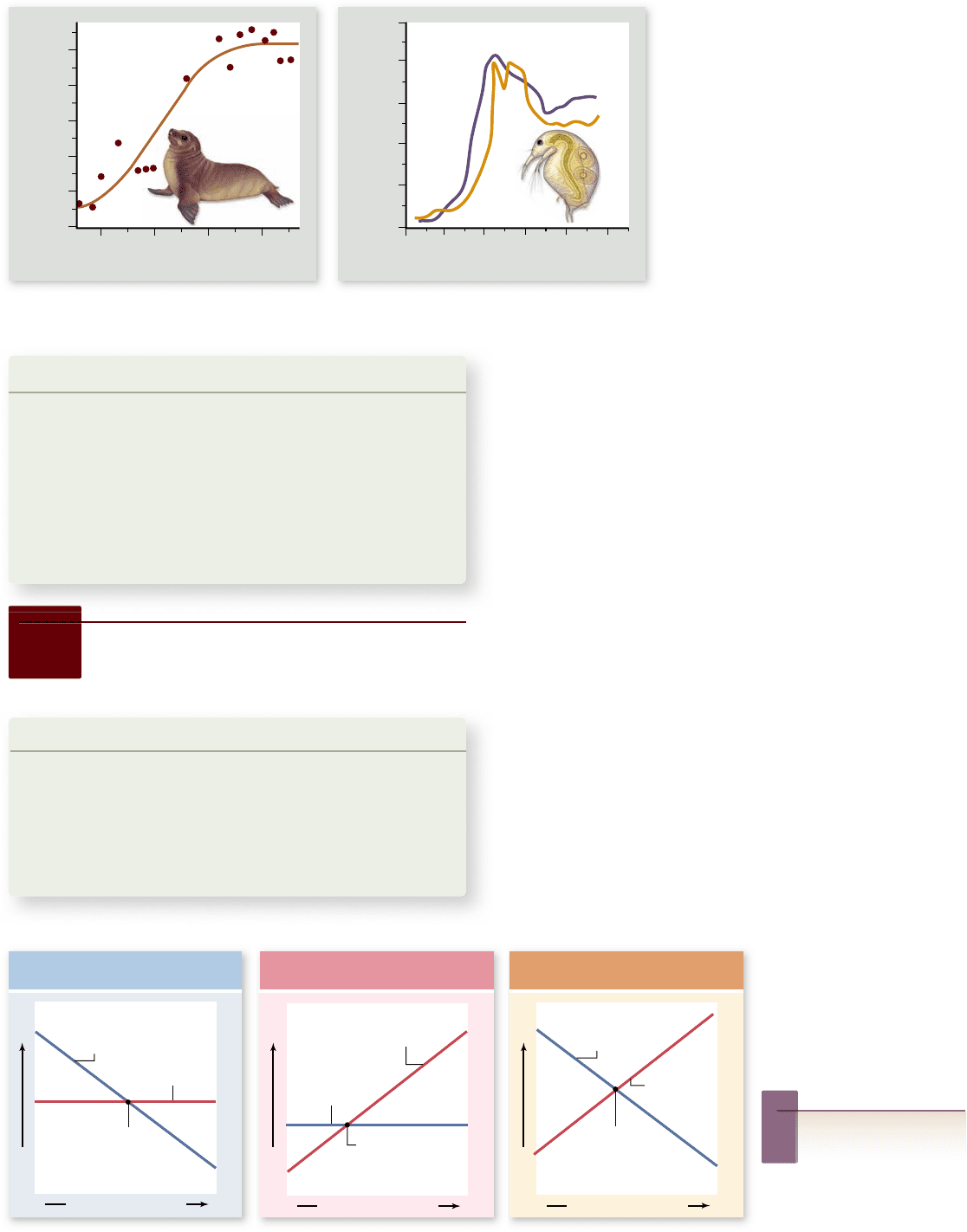
Time (years)
Number of Breeding Male
Fur Seals (thousands)
1915 1925 1935 1945
a. b.
20 0 10 30 50 40
10
8
6
4
2
0
Number of Cladocerans (per 200 mL)
Time (days)
500
400
300
200
100
0
HighLow
HighLow
HighLow
Density-
dependent
birth rate
Density-
dependent
death rate
Equilibrium
population
density
Density-
dependent
bir
th rate
Density-
independent
death rate
Equilibrium
population
density
Affecting Birth and Death Rates
Population Density
Affecting Birth Rates
Population Density
Affecting Death Rates
Population Density
Density-
independent
bir
th rate
Density-
dependent
death rate
Equilibrium
population
density
Figure 56.19
Density-
dependent population
regulation. Density-
dependent factors can affect
birth rates, death rates,
or both.
Inquiry question
?
Why might birth rates
be density-dependent?
Figure 56.18
Many populations
exhibit logistic growth.
a. A fur seal
(Callorhinus ursinus) population on St. Paul
Island, Alaska. b. Two laboratory
populations of the cladoceran Bosmina
longirostris. Note that the populations rst
exceeded the carrying capacity, before
decreasing to a size that was then
maintained.
Learning Outcomes Review 56.5
Exponential growth refers to population growth in which the number of
individuals accelerates even when the rate of increase remains constant; it
results in a population explosion. Exponential growth is eventually limited
by resource availability. The size at which a population in a particular location
stabilizes is defi ned as the carrying capacity of that location for that species.
Populations often grow to the carrying capacity of their environment.
■ What might cause a population’s carrying capacity to
change, and how would the population respond?
56.6
Factors That Regulate
Populations
Learning Outcomes
Compare density-dependent and density-independent 1.
factors.
Evaluate why the size of some populations cycle.2.
Consider how the life history adaptations of species may 3.
differ depending on how often populations are at their
carrying capacity.
A number of factors may affect population size through time.
Some of these factors depend on population size and are there-
fore termed density-dependent. Other factors, such as natural di-
sasters, affect populations regardless of size; these factors are
termed density-independent. Many populations exhibit cyclic
fluctuations in size that may result from complex interactions
of factors.
Density-dependent e ects occur when
reproduction and survival are a ected
by population size
The reason population growth rates are affected by population
size is that many important processes have density-dependent
effects. That is, as population size increases, either reproduc-
tive rates decline or mortality rates increase, or both, a phe-
nomenon termed negative feedback (figure 56.19).
Populations can be regulated in many different ways.
When populations approach their carrying capacity, compe-
tition for resources can be severe, leading both to a decreased
birth rate and an increased risk of death (figure 56.20) . In
addition, predators often focus their attention on a particu-
larly common prey species, which also results in increasing
rates of mortality as populations increase. High population
densities can also lead to an accumulation of toxic wastes in
the environment.
chapter
56
Ecology of Individuals and Populations
1175www.ravenbiology.com
rav32223_ch56_1162-1184.indd 1175rav32223_ch56_1162-1184.indd 1175 11/20/09 1:47:07 PM11/20/09 1:47:07 PM
Apago PDF Enhancer
Panolis
Hyloicus
Dendrolimus
Bupalus
Number of Moth Pupae per m
2
Plotted on a Logarithmic Scale
10
3
10
10
3
10
10
5
10
3
10
10
5
10
3
10
1880 1890 1910 1930 1900 1920 1940
Year
0.4
0.5
0.7
0.6
0.8
0.9
40 80
Number of Breeding Adults
120
100 60 20 0
140
2.0
1.0
3.0
4.0
5.0
Juvenile Mortality
Number of Young per Female
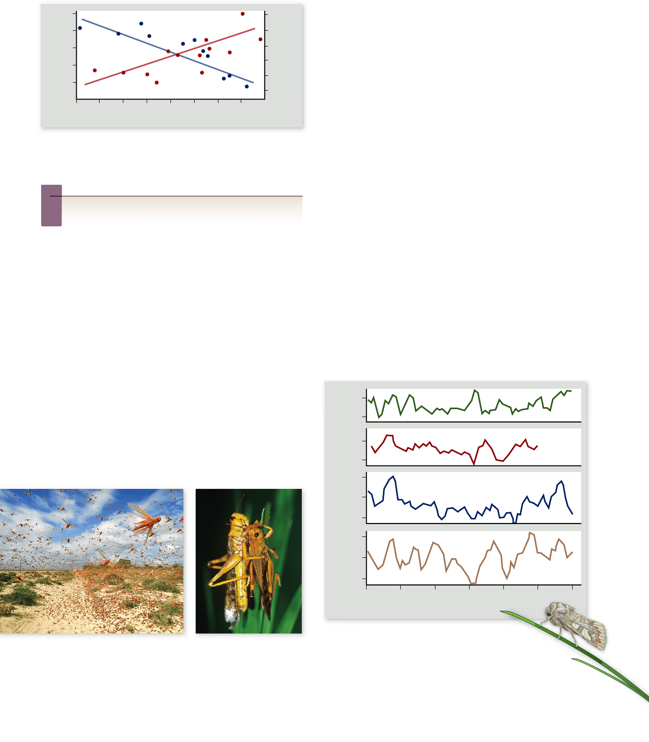
Figure 56.20
Density dependence in the song sparrow
(Melospiza melodia) on Mandarte Island. Reproductive success
decreases and mortality rates increase as population size increases.
Inquiry question
?
What would happen if researchers supplemented the food
available to the birds?
Figure 56.21
Density-dependent e ects. Migratory
locusts (Locusta migratoria) are a legendary plague of large areas of
Africa and Eurasia. At high population densities, the locusts have
different hormonal and physical characteristics and take off as
a swarm.
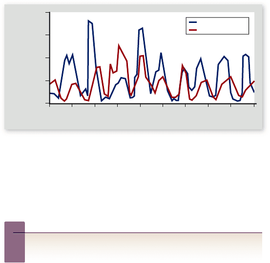
Figure 56.22
Fluctuations in the number
of pupae of four moth species in Germany. The
population uctuations suggest that density-independent
factors are regulating population size. The concordance in trends
through time suggests that the same factors are regulating
population size in all four species.
Behavioral changes may also affect population growth
rates. Some species of rodents, for example, become antisocial,
fighting more, breeding less, and generally acting stressed-out.
These behavioral changes result from hormonal actions, but
their ultimate cause is not yet clear; most likely, they have
evolved as adaptive responses to situations in which resources
are scarce. In addition, in crowded populations, the population
growth rate may decrease because of an increased rate of emi-
gration of individuals attempting to find better conditions else-
where (figure 56.21).
However, not all density-dependent factors are negatively
related to population size. In some cases, growth rates increase
with population size. This phenomenon is referred to as the Allee
effect (after Warder Allee, who first described it), and is an ex-
ample of positive feedback. The Allee effect can take several forms.
Most obviously, in populations that are too sparsely distributed,
individuals may have difficulty finding mates. Moreover, some
species may rely on large groups to deter predators or to provide
the necessary stimulation for breeding activities. The Allee effect
is a major threat for many endangered species, which may never
recover from decreased population sizes caused by habitat de-
struction, overexploitation, or other causes (see chapter 60).
Density-independent e ects include
environmental disruptions and catastrophes
Growth rates in populations sometimes do not correspond to the
logistic growth equation. In many cases, such patterns result be-
cause growth is under the control of density-independent effects.
In other words, the rate of growth of a population at any instant is
limited by something unrelated to the size of the population.
A variety of factors may affect populations in a density-
independent manner. Most of these are aspects of the external
environment, such as extremely cold winters, droughts, storms,
or volcanic eruptions. Individuals often are affected by these
occurrences regardless of the size of the population.
Populations in areas where such events occur relatively fre-
quently display erratic growth patterns in which the populations
increase rapidly when conditions are benign, but exhibit large re-
ductions whenever the environment turns hostile (figure 56.22) .
Needless to say, such populations do not produce the sigmoidal
growth curves characteristic of the logistic equation.
Population cycles may re ect
complex interactions
In some populations, density-dependent effects lead not to an
equilibrium population size but to cyclic patterns of increase
and decrease. For example, ecologists have studied cycles in hare
117 6
part
VIII
Ecology and Behavior
rav32223_ch56_1162-1184.indd 1176rav32223_ch56_1162-1184.indd 1176 11/20/09 1:47:08 PM11/20/09 1:47:08 PM
Apago PDF Enhancer
1845 1855 1865
1875 1885 1895 1905 1915 1925 1935
40
0
80
120
160
Year
Number of Pelts (in thousands)
snowshoe hare
lynx
Figure 56.23
Linked population cycles of the snowshoe
hare (Lepus americanus) and the northern lynx (Lynx
canadensis). These data are based on records of fur returns from
trappers in the Hudson Bay region of Canada. The lynx population
carefully tracks that of the snowshoe hare, but lags behind it
slightly.
Inquiry question
?
Suppose experimenters artificially kept the hare population
at a high and constant level; what would happen to the lynx
population? Conversely, if experimenters artificially kept the
lynx population at a high and constant level, what would
happen to the hare population?
In Canada’s Yukon, Krebs set up experimental plots that
contained hare populations. If food is added (no food shortage
effect) and predators are excluded (no predator effect) in an
experimental area, hare numbers increase 10-fold and stay
there—the cycle is lost. However, the cycle is retained if either
of the factors is allowed to operate alone: exclude predators but
don’t add food (food shortage effect alone), or add food in the
presence of predators (predator effect alone). Thus, both fac-
tors can affect the cycle, which in practice seems to be gener-
ated by the interaction between the two.
Population cycles traditionally have been considered to
occur rarely. However, a recent review of nearly 700 long-term
(25 years or more) studies of trends within populations found
that cycles were not uncommon; nearly 30% of the studies—
including birds, mammals, fish, and crustaceans—provided evi-
dence of some cyclic pattern in population size through time,
although most of these cycles are nowhere near as dramatic in
amplitude as the hare–lynx cycles. In some cases, such as that of
the snowshoe hare and lynx, density-dependent factors may be
involved, whereas in other cases, density-independent factors,
such as cyclic climatic patterns, may be responsible.
Resource availability a ects
life history adaptations
As you have seen, some species usually maintain stable popula-
tion sizes near the carrying capacity, whereas in other species
population sizes fluctuate markedly and are often far below car-
rying capacity. The selective factors affecting such species differ
markedly. Individuals in populations near their carrying capac-
ity may face stiff competition for limited resources; by contrast,
individuals in populations far below carrying capacity have ac-
cess to abundant resources.
We have already described the consequences of such dif-
ferences. When resources are limited, the cost of reproduction
often will be very high. Consequently, selection will favor indi-
viduals that can compete effectively and utilize resources effi-
ciently. Such adaptations often come at the cost of lowered
reproductive rates. Such populations are termed K-selected be-
cause they ar e adapted to thrive when the population is near its
carrying capacity (K). Table 56.3 lists some of the typical features
of K-selected populations. Examples of K-selected species in-
clude coconut palms, whooping cranes, whales, and humans.
By contrast, in populations far below the carrying capac-
ity, resources may be abundant. Costs of reproduction are low,
and selection favors those individuals that can produce the
maximum number of offspring. Selection here favors individu-
als with the highest reproductive rates; such populations are
termed r-selected. Examples of organisms displaying r- selected
life history adaptations include dandelions, aphids, mice,
and cockroaches.
Most natural populations show life history adaptations
that exist along a continuum ranging from completely
r-selected traits to completely K-selected traits. Although these
tendencies hold true as generalities, few populations are purely
r- or K-selected and show all of the traits listed in table 56.3.
These attributes should be treated as generalities, with the rec-
ognition that many exceptions exist.
populations since the 1820s. They have found that the North
American snowshoe hare (Lepus americanus) follows a “10-year
cycle” (in reality, the cycle varies from 8 to 11 years). Hare popu-
lation numbers fall 10-fold to 30-fold in a typical cycle, and 100-
fold changes can occur (figure 56.23). Two factors appear to be
generating the cycle: food plants and predators.
Food plants. The preferred foods of snowshoe hares are willow
and birch twigs. As hare density increases, the quantity of
these twigs decreases, forcing the hares to feed on
high- ber (low-quality) food. Lower birthrates, low
juvenile survivorship, and low growth rates follow. The
hares also spend more time searching for food, an activity
that increases their exposure to predation. The result is a
precipitous decline in willow and birch twig abundance,
and a corresponding fall in hare abundance. It takes 2 to
3 years for the quantity of mature twigs to recover.
Predators. A key predator of the snowshoe hare is the
Canada lynx. The Canada lynx shows a “10-year” cycle
of abundance that seems remarkably entrained to the
hare abundance cycle (see gure 55.23). As hare
numbers increase, lynx numbers do too, rising in
response to the increased availability of the lynx’s food.
When hare numbers fall, so do lynx numbers, their food
supply depleted.
Which factor is responsible for the predator–prey oscilla-
tions? Do increasing numbers of hares lead to overharvesting
of plants (a hare–plant cycle), or do increasing numbers of lynx
lead to overharvesting of hares (a hare–lynx cycle)? Field ex-
periments carried out by Charles Krebs and coworkers in 1992
provide an answer.
chapter
56
Ecology of Individuals and Populations
117 7www.ravenbiology.com
rav32223_ch56_1162-1184.indd 1177rav32223_ch56_1162-1184.indd 1177 11/20/09 1:47:09 PM11/20/09 1:47:09 PM

Apago PDF Enhancer
Learning Outcomes Review 56.6
Density-dependent factors such as resource availability come into play
particularly when population size is larger; density-independent factors
such as natural disasters operate regardless of population size. Population
density may be cyclic due to complex interactions such as resource cycles and
predator eff ects. Populations with density-dependent regulation often are
near their carrying capacity; in species with populations well below carrying
capacity, natural selection may favor high rates of reproduction when
resources are abundant.
■ Can a population experience both positive and negative
density-dependent effects?
TABLE 56.3
r-Selected and K-Selected Life
History Adaptations
Adaptation
r-Selected
Populations
K-Selected
Populations
Age at rst reproduction Early Late
Life span Short Long
Maturation time Short Long
Mortality rate Often high Usually low
Number of o spring
produced per repro ductive
episode
Many Few
Number of reproductions
per lifetime
Few Many
Parental care None Often extensive
Size of o spring or eggs Small Large
56.7
Human Population Growth
Learning Outcomes
Explain how the rate of human population growth has 1.
changed through time.
Describe the effects of age distribution on future growth.2.
Evaluate the relative importance of rapid population 3.
growth and resource consumption as threats to the
biosphere and human welfare.
Humans exhibit many K-selected life history traits, including
small brood size, late reproduction, and a high degree of paren-
tal care. These life history traits evolved during the early his-
tory of hominids, when the limited resources available from the
environment controlled population size. Throughout most of
human history, our populations have been regulated by food
availability, disease, and predators. Although unusual distur-
bances, including floods, plagues, and droughts, no doubt af-
fected the pattern of human population growth, the overall size
of the human population grew slowly during our early history.
Two thousand years ago, perhaps 130 million people pop-
ulated the Earth. It took a thousand years for that number to
double, and it was 1650 before it had doubled again, to about
500 million. In other words, for over 16 centuries, the human
population was characterized by very slow growth. In this re-
spect, human populations resembled many other species with
predominantly K-selected life history adaptations.
Human populations have
grown exponentially
Starting in the early 1700s, changes in technology gave humans
more control over their food supply, enabled them to develop
superior weapons to ward off predators, and led to the develop-
ment of cures for many diseases. At the same time, improve-
ments in shelter and storage capabilities made humans less
vulnerable to climatic uncertainties. These changes allowed hu-
mans to expand the carrying capacity of the habitats in which
they lived and thus to escape the confines of logistic growth and
re-enter the exponential phase of the sigmoidal growth curve.
Responding to the lack of environmental constraints, the
human population has grown explosively over the last 300
years. Although the birth rate has remained unchanged at about
30 per 1000 per year over this period, the death rate has fallen
dramatically, from 20 per 1000 per year to its present level of 13
per 1000 per year. The difference between birth and death rates
meant that the population grew as much as 2% per year, al-
though the rate has now declined to 1.2% per year.
A 1.2% annual growth rate may not seem large, but it has
produced a current human population of nearly 7 billion people
(figure 56.24) . At this growth rate, 78 million people would be
added to the world population in the next year, and the human
population would double in 58 years. Both the current human
population level and the projected growth rate have potentially
grave consequences for our future.
Population pyramids show
birth and death trends
Although the human population as a whole continues to grow
rapidly at the beginning of the 21st century, this growth is not
occurring uniformly over the planet. Rather, most of the popu-
lation growth is occurring in Africa, Asia, and Latin America
(figure 56.25) . By contrast, populations are actually decreasing
in some countries in Europe.
The rate at which a population can be expected to grow in
the future can be assessed graphically by means of a population
pyramid, a bar graph displaying the numbers of people in each
age category (figure 56.26) . Males are conventionally shown to
the left of the vertical age axis, females to the right. A human
population pyramid thus displays the age composition of a popu-
lation by sex. In most human population pyramids, the number
of older females is disproportionately large compared with the
117 8
part
VIII
Ecology and Behavior
rav32223_ch56_1162-1184.indd 1178rav32223_ch56_1162-1184.indd 1178 11/20/09 1:47:10 PM11/20/09 1:47:10 PM
Apago PDF Enhancer
4000
B.C.
2
1
3
4
5
6
3000
B.C.
2000
B.C.
1000
B.C.
Year
Industrial
Revolution
Significant advances
in public health
Bubonic plague
“Black Death”
Billions of People
0 1000 2000
0
200
400
600
800
1000
1200
1400
1600
1800
2000
5000
6000
7000
Population (in millions)
North
America
Europe Australasia
South
America
Africa Asia
907
1931
871
767
2005
2050
33
5350
6721
48
516
685
375
527
male
female
80;
65–69
75–79
55–59
60–64
50–54
70–74
40–44
45–49
35–39
25–29
30–34
20–24
10–14
15–19
0–4
5–9
Percent of Population
Age
KenyaSweden
0396 369121518 1812 1504848
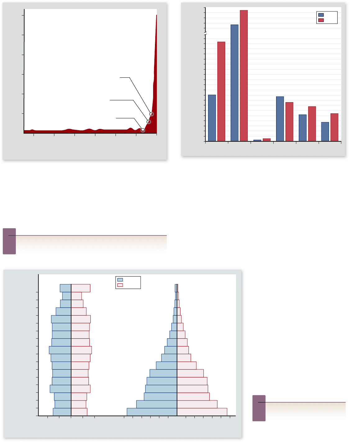
Figure 56.24
History of human population size.
Temporary increases in death rate, even a severe one such as that
occurring during the Black Death of the 1300s, have little lasting
effect. Explosive growth began with the Industrial Revolution in
the 1800s, which produced a signi cant, long-term lowering of the
death rate. The current world population is 6.9 billion, and at the
present rate, it will double in 58 years.
Inquiry question
?
Based on what we have learned about population growth,
what do you predict will happen to human population size?
Figure 56.26
Population
pyramids from 2008. Population
pyramids are graphed according to a
population’s age distribution. Kenya’s
pyramid has a broad base because of
the great number of individuals below
childbearing age. When the young
people begin to bear children, the
population will experience rapid
growth. The Swedish pyramid
exhibits a slight bulge among middle-
aged Swedes, the result of the “baby
boom” that occurred in the middle of
the 20th century, and many
postreproductive individuals resulting
from Sweden’s long average life span.
Inquiry question
?
What will the population
distributions look like in
20 years?
Figure 56.25
Projected p opulation growth in 2050.
Developed countries are predicted to grow little; almost all of the
population increase will occur in less-developed countries.
number of older males, because females in most regions have a
longer life expectancy than males.
Viewing such a pyramid, we can predict demographic
trends in births and deaths. In general, a rectangular pyramid is
characteristic of countries whose populations are stable, neither
growing nor shrinking. A triangular pyramid is characteristic of
a country that will exhibit rapid future growth because most of
chapter
56
Ecology of Individuals and Populations
117 9www.ravenbiology.com
rav32223_ch56_1162-1184.indd 1179rav32223_ch56_1162-1184.indd 1179 11/20/09 1:47:11 PM11/20/09 1:47:11 PM
Apago PDF Enhancer
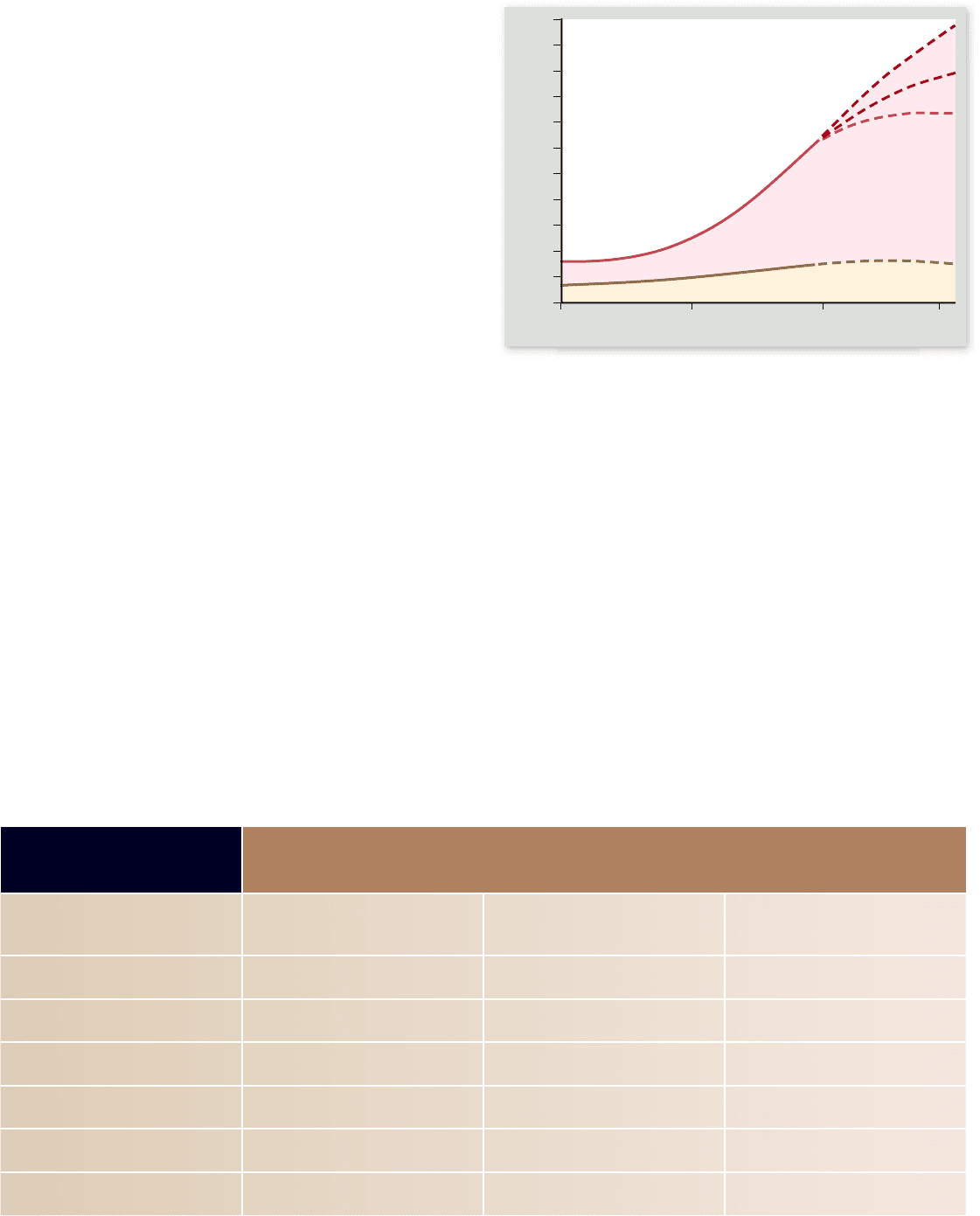
1
2
3
Time
World Population in Billions
1950 1900 2000
Developing countries
World total
2050
4
5
6
7
8
9
10
11
0
Developed countries
h
i
g
h
f
e
r
t
i
l
i
t
y
low fertility
m
e
d
i
u
m
f
e
r
t
i
l
i
t
y
In the future, the world’s population growth will be centered in
the parts of the world least equipped to deal with the pressures
of rapid growth.
Rapid population growth in developing countries has had
the harsh consequence of increasing the gap between rich and
poor. Today, the 19% of the world’s population that lives in the
industrialized world have a per capita income of $22,060, but
81% of the world’s population lives in developing countries and
has a per capita income of only $3,580. Furthermore, of the
its population has not yet entered the childbearing years. In-
verted triangles are characteristic of populations that are shrink-
ing, usually as a result of sharply declining birth rates.
Examples of population pyramids for Sweden and Kenya
in 2008 are shown in figure 56.26. The two countries exhibit
very different age distributions. The nearly rectangular popula-
tion pyramid for Sweden indicates that its population is not
expanding because birth rates have decreased and average life
span has increased. The very triangular pyramid of Kenya, by
contrast, results from relatively high birthrates and shorter av-
erage life spans, which can lead to explosive future growth. The
difference is most apparent when we consider that only 16% of
Sweden’s population is less than 15 years old, compared with
nearly half of all Kenyans. Moreover, the fertility rate (offspring
per woman) in Sweden is 1.7; in Kenya, it is 4.7. As a result,
Kenya’s population could double in less than 35 years, whereas
Sweden’s will remain stable.
Humanity’s future growth is uncertain
Earth’s rapidly growing human population constitutes per-
haps the greatest challenge to the future of the biosphere, the
world’s interacting community of living things. Humanity is
adding 78 million people a year to its population—over a mil-
lion every 5 days, 150 every minute! In more rapidly growing
countries, the resulting population increase is staggering
(table 56.4) . India, for example, had a population of 1.05 bil-
lion in 2002; by 2050, its population likely will exceed
1.6 billion.
A key element in the world’s population growth is its un-
even distribution among countries. Of the billion people added
to the world’s population in the 1990s, 90% live in developing
countries (figure 56.27) . The fraction of the world’s population
that lives in industrialized countries is therefore diminishing. In
1950, fully one-third of the world’s population lived in industri-
alized countries; by 1996, that proportion had fallen to one-
quarter; and in 2020, the proportion will have fallen to one-sixth.
Figure 56.27
Distribution of population growth. Most
of the worldwide increase in population since 1950 has occurred in
developing countries. The age structures of developing countries
indicate that this trend will increase in the near future. World
population in 2050 likely will be between 7.3 and 10.7 billion,
according to a recent United Nations study. Depending on fertility
rates, the population at that time will either be increasing rapidly or
slightly, or in the best case, declining slightly.
TABLE 56.4
A Comparison of 2005 Population Data in Developed
and Developing Countries
United States
(highly developed)
Brazil
(moderately developed)
Ethiopia
(poorly developed)
Fertility rate 2.1 1.9 5.3
Doubling time at current rate (years) 75 65 29
Infant mortality rate (per 1000 births) 6.5 30 95
Life expectancy at birth (years) 78 72 49
Per capita GDP (U.S. $)* $40,100 $8100 $800
Population < 15 years old (%) 21 26 44
*GDP, gross domestic product.
118 0
part
VIII
Ecology and Behavior
rav32223_ch56_1162-1184.indd 1180rav32223_ch56_1162-1184.indd 1180 11/20/09 1:47:11 PM11/20/09 1:47:11 PM
Apago PDF Enhancer
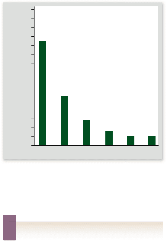
23.2
10.4
5.9
3.2
2.2 2.2
2
0
4
6
8
12
10
14
16
18
20
22
24
26
28
30
USA
Germany
Acres of Land Required to Support an
Individual at Standard of Living of Population
Brazil
Indonesia
Nigeria
India
Figure 56.28
Ecological footprints of individuals in
di erent countries. An ecological footprint calculates how much
land is required to support a person through his or her life,
including the acreage used for production of food, forest products,
and housing, in addition to the forest required to absorb the carbon
dioxide produced by the combustion of fossil fuels.
Inquiry question
?
Which is a more important cause of resource depletion,
overpopulation or overconsumption?
Consumption in the developed
world further depletes resources
Population size is not the only factor that determines resource use;
per capita consumption is also important. In this respect, we in the
industrialized world need to pay more attention to lessening the
impact each of us makes because, even though the vast majority of
the world’s population is in developing countries, the overwhelm-
ing percentage of consumption of resources occurs in the industri-
alized countries. Indeed, the wealthiest 20% of the world’s
population accounts for 86% of the world’s consumption of re-
sources and produces 53% of the world’s carbon dioxide emissions,
whereas the poorest 20% of the world is responsible for only 1.3%
of consumption and 3% of carbon dioxide emissions. Looked at
another way, in terms of resource use, a child born today in the in-
dustrialized world will consume many more resources over the
course of his or her life than a child born in the developing world.
One way of quantifying this disparity is by calculating what
has been termed the ecological footprint, which is the amount of
productive land required to support an individual at the standard of
living of a particular population through the course of his or her
life. This figure estimates the acreage used for the production of
food (both plant and animal), forest products, and housing, as well
as the area of forest required to absorb carbon dioxide produced by
the combustion of fossil fuels. As figure 56.28 illustrates, the
people in the developing world, about one-quarter of the popu-
lation gets by on $1 per day. Eighty percent of all the energy
used today is consumed by the industrialized world, but only
20% is used by developing countries.
No one knows whether the world can sustain today’s pop-
ulation of 6.9 billion people, much less the far greater numbers
expected in the future. As chapter 58 outlines, the world ecosys-
tem is already under considerable stress. We cannot reasonably
expect to expand its carrying capacity indefinitely, and indeed
we already seem to be stretching the limits.
Despite using an estimated 45% of the total biological
productivity of Earth’s landmasses and more than one-half of
all renewable sources of fresh water, between one-fourth and
one-eighth of all people in the world are malnourished. More-
over, as anticipated by Thomas Malthus in his famous 1798
work, Essay on the Principle of Population, death rates are begin-
ning to rise in some areas. In sub-Saharan Africa, for example,
population projections for the year 2025 have been scaled back
from 1.33 billion to 1.05 billion (21%) because of the effect of
AIDS. Similar decreases are projected for Russia as a result of
higher death rates due to disease.
If we are to avoid catastrophic increases in the death
rate, birth rates must fall dramatically. Faced with this grim
dichotomy, significant efforts are underway worldwide to
lower birth rates.
The population growth
rate has declined
The world population growth rate is declining, from a high of
2.0% in the period 1965–1970 to 1.2% in 2008 . Nonetheless,
because of the larger population, this amounts to an increase of
78 million people per year to the world population, compared
with 53 million per year in the 1960s.
The United Nations attributes the growth rate decline to
increased family planning efforts and the increased economic
power and social status of women. The United States has led
the world in funding family planning programs abroad, but
some groups oppose spending money on international family
planning. The opposition believes that money is better spent
on improving education and the economy in other countries,
leading to an increased awareness and lowered fertility rates.
The U.N. certainly supports the improvement of education
programs in developing countries, but interestingly, it has re-
ported increased education levels following a decrease in family
size as a result of family planning.
Most countries are devoting considerable attention to
slowing the growth rate of their populations, and there are
genuine signs of progress. For example, from 1984 to 2008 ,
family planning programs in Kenya succeeded in reducing the
fertility rate from 8.0 to 4.7 children per couple, thus lowering
the population growth rate from 4.0% per year to 2.8% per
year. Because of these efforts, the global population may stabi-
lize at about 8.9 billion people by the middle of the current
century. How many people the planet can support sustainably
depends on the quality of life that we want to achieve; there are
already more people than can be sustainably supported with
current technologies.
chapter
56
Ecology of Individuals and Populations
118 1www.ravenbiology.com
rav32223_ch56_1162-1184.indd 1181rav32223_ch56_1162-1184.indd 1181 11/20/09 1:47:11 PM11/20/09 1:47:11 PM