Raven P.H., Johnson G.B., Mason K.A. Biology (Ninth Edition)
Подождите немного. Документ загружается.

Apago PDF Enhancer
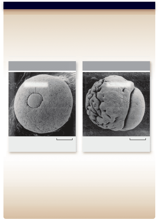
Hypothesis: Fibronectin is required for cell migration during gastrulation.
Prediction: Blocking bronectin with antibronectin antibodies before
gastrulation should prevent cell movement.
Test: Staged salamander embryos were injected either with
antibronectin antibody, or with preimmune serum as a control, prior to
gastrulation. Cell movements were then monitored photographically.
Result: The experimental embryos injected with antibronectin antibody
show extremely aberrant gastrulation where cells pile up and do not enter
the interior of the embryo. Control embryos gastrulate normally.
Conclusion: Fibronectin is required for cells to migrate into the interior
of the embryo during gastrulation.
Further Experiments: How can this same system be used to analyze
the role of bronectin in other early morphogenetic events?
SCI ENT I FI C THINKING
a. b.
285.7 µm285.7 µm
BlastoporeBlastopore
Cells have moved
into the interior
Cells pile up on
the surface
Treated with AntifibronectinTreated with Preimmune
Figure 19.20
Fibronectin is necessary for cell migration
during gastrulation.
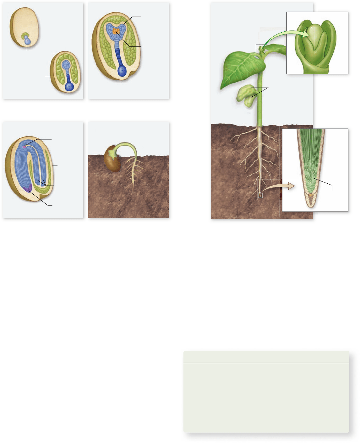
cells is small, with dense cytoplasm (figure 19.21a). That
cell, the future embryo, begins to divide repeatedly, forming
a ball of cells. The other daughter cell also divides repeat-
edly, forming an elongated structure called a suspensor, which
links the embryo to the nutrient tissue of the seed. The sus-
pensor also provides a route for nutrients to reach the devel-
oping embryo.
Just as many animal embryos acquire their initial axis as a
cell mass formed during cleavage divisions, so the plant embryo
forms its root–shoot axis at this time. Cells near the suspensor
are destined to form a root, whereas those at the other end of
the axis ultimately become a shoot, the aboveground portion of
the plant.
The relative position of cells within the plant embryo is
also a primary determinant of cell differentiation. The outer-
most cells in a plant embryo become epidermal cells. The bulk
of the embryonic interior consists of ground tissue cells that
eventually function in food and water storage. Finally, cells at
the core of the embryo are destined to form the future vascular
tissue (figure 19.21b). (Plant tissues and development are de-
scribed in detail in chapters 36 and 37.)
An example of the action of cadherins can be seen in the
development of the vertebrate nervous system. All surface ec-
toderm cells of the embryo express E-cadherin. The formation
of the nervous system begins when a central strip of cells on
the dorsal surface of the embryo turns off E-cadherin expres-
sion and turns on N-cadherin expression. In the process of
neurulation, the formation of the neural tube (see chapter 54) ,
the central strip of N-cadherin-expressing cells folds up to
form the tube. The neural tube pinches off from the overlying
cells, which continue to express E-cadherin. The surface cells
outside the tube differentiate into the epidermis of the skin,
whereas the neural tube develops into the brain and spinal
cord of the embryo.
Integrins
In some tissues, such as connective tissue, much of the volume
of the tissue is taken up by the spaces between cells. These spaces
are filled with a network of molecules secreted by surrounding
cells, termed a matrix. In connective tissue such as cartilage,
long polysaccharide chains are covalently linked to proteins
(proteoglycans), within which are embedded strands of fibrous
protein (collagen, elastin, and fibronectin). Migrating cells tra-
verse this matrix by binding to it with cell surface proteins
called integrins .
Integrins are attached to actin filaments of the cytoskel-
eton and protrude out from the cell surface in pairs, like two
hands. The “hands” grasp a specific component of the matrix,
such as collagen or fibronectin, thus linking the cytoskeleton to
the fibers of the matrix. In addition to providing an anchor, this
binding can initiate changes within the cell, alter the growth of
the cytoskeleton, and activate gene expression and the produc-
tion of new proteins.
The process of gastrulation (described in detail in chap-
ter 54) , during which the hollow ball of animal embryonic cells
folds in on itself to form a multilayered structure, depends on
fibronectin–integrin interactions. For example, injection of an-
tibodies against either fibronectin or integrins into salamander
embryos blocks binding of cells to fibronectin in the ECM and
inhibits gastrulation. The result is like a huge traffic jam fol-
lowing a major accident on a freeway: Cells (cars) keep coming,
but they get backed up since they cannot get beyond the area of
inhibition (accident site) (figure 19.20). Similarly, a targeted
knockout of the fibronectin gene in mice resulted in gross de-
fects in the migration, proliferation, and differentiation of em-
bryonic mesoderm cells.
Thus, cell migration is largely a matter of changing pat-
terns of cell adhesion. As a migrating cell travels, it continually
extends projections that probe the nature of its environment.
Tugged this way and that by different tentative attachments,
the cell literally feels its way toward its ultimate target site.
In seed plants, the plane of cell division
determines morphogenesis
The form of a plant body is largely determined by the plane
in which cells divide. The first division of the fertilized egg
in a flowering plant is off-center, so that one of the daughter
392
part
III
Genetic and Molecular Biology
rav32223_ch19_372-395.indd 392rav32223_ch19_372-395.indd 392 11/10/09 4:28:57 PM11/10/09 4:28:57 PM
Apago PDF Enhancer
a. Early cell division
Embryo
Embryo
Suspensor
b. Tissue formation
d. Germination c. Seed formation
Seed wall
Shoot apical
mer
istem
Root apical
meristem
Shoot apical meristem
Cotyledons
e. Meristematic development and morphogenesis
Root apical
mer
istem
Epidermal
cells
Ground
tissue cells
Vascular
tissue cells
Cotyledons
Soon after the three basic tissues form, a flowering
plant embryo develops one or two seed leaves called cotyle-
dons. At this point, development is arrested, and the embryo
is either surrounded by nutritive tissue or has amassed stored
food in its cotyledons (figure 19.21c). The resulting package,
known as a seed, is resistant to drought and other unfavor-
able conditions.
A seed germinates in response to favorable changes in its
environment. The embryo within the seed resumes develop-
ment and grows rapidly, its roots extending downward and its
leaf-bearing shoots extending upward (figure 19.21d). Plant de-
velopment exhibits its great flexibility during the assembly of
the modules that make up a plant body. Apical meristems at the
root and shoot tips generate the large numbers of cells needed
to form leaves, flowers, and all other components of the mature
plant (figure 19.21e).
Growth within the developing flower is controlled by a
cascade of transcription factors. A key member of this cascade
is the AINTEGUMENTA (ANT) gene. Loss of ANT function
reduces the number and size of floral organs, and inappropriate
expression leads to larger floral organs.
Plant body form is also established by controlled changes
in cell shape as cells expand osmotically after they form. Plant
growth-regulating hormones and other factors influence the
orientation of bundles of microtubules on the interior of the
plasma membrane. These microtubules seem to guide cellulose
deposition as the cell wall forms around the outside of a new
cell. The orientation of the cellulose fibers, in turn, determines
how the cell will elongate as it increases in volume due to os-
mosis, and so determines the cell’s final shape.
Learning Outcomes Review 19.6
Morphogenesis is the generation of ordered form and structure. This
process proceeds along with cell diff erentiation. The primary mechanisms
of morphogenesis are cell shape change and cell migration. Apoptosis is
programmed cell death that is a necessary part of morphogenesis. Cell
migration in animals involves alternating changes in adhesion brought
about by cadherins and integrins. In plants, which cannot move, cell division
and cell expansion are the primary morphogenetic processes.
■ Why is cell death important to morphogenesis?
Figure 19.21
The path of plant development. The developmental stages of Arabidopsis thaliana are (a) early embryonic cell division,
(b) embryonic tissue formation, (c) seed formation, (d) germination, and (e) meristematic development and morphogenesis.
chapter
19
Cellular Mechanisms of Development
393www.ravenbiology.com
rav32223_ch19_372-395.indd 393rav32223_ch19_372-395.indd 393 11/10/09 4:29:01 PM11/10/09 4:29:01 PM
Apago PDF Enhancer
Nuclear reprogramming has been accomplished by use of
de ned factors.
Adult cells can be converted into pluripotent cells by introduction of
four genes for transcription factors. These induced pluripotent cells
appear to be similar to ES cells.
The use of cells cloned from a patient’s cells to replace damaged
tissue could avoid the problem of transplant rejection.
19.5 Pattern Formation
Drosophila embryogenesis produces a segmented larva.
The maternal contribution of mRNA along with the postfertilization
events of cellular blastoderm formation produce a segmented embryo.
Morphogen gradients form the basic body axes in Drosophila.
Pattern formation produces two perpendicular axes in a bilaterally
symmetrical organism. Positional information leads to changes in
gene activity so cells adopt a fate appropriate for their location.
Formation of the anterior/posterior (A/P) axis is based on opposing
gradients of morphogens, Bicoid and Nanos, synthesized from
maternal mRNA ( gures 19.14, 19.15).
The dorsal/ventral (D/V) axis is established by a gradient of the
Dorsal transcription factor. Successive action of transcription factors
divides the embryo into segments.
The body plan is produced by sequential activation of genes.
Segment identity arises from the action of homeotic genes.
Homeotic genes, called Hox genes because they contain a DNA
sequence called the homeobox, give identity to embryo segments.
Hox genes are found in four clusters in vertebrates.
Pattern formation in plants is also under genetic control.
Plants have MADS-box genes that control the transition from vegetative
to reproductive growth, root development, and oral organ identity.
19.6 Morphogenesis
Cell division during development may result in unequal cytokinesis.
Cells change shape and size as morphogenesis proceeds.
Depending on the orientation of the mitotic spindle, cells
of equal or different sizes can arise. Morphogenesis involves changes
in cell shape and size and cell migration.
Programmed cell death is a necessary part of development.
Apoptosis, the programmed death of cells, removes structures once
they are no longer needed ( gure 19.19).
Cell migration gets the right cells to the right places.
The migration of cells requires both adhesion and loss of adhesion
between cells and their substrate.
Cell-to-cell interactions are often mediated by cadherin proteins,
whereas cell-to-substrate interactions may involve integrin-to-
extracellular-matrix interactions.
Integrins bind to bers found in the extracellular matrix. This action
can alter the cytoskeleton and activate gene expression.
In seed plants, the plane of cell division determines morphogenesis.
In plants, the primary morphogenetic processes are cell division,
relative position of cells within the embryo, and changes in cell
shape. Plant development stages begin with cell division and end with
meristematic development and morphogenesis ( gure 19.21).
Relative position of cells in the plant embryo is the main determinant
of cell differentiation.
19.1 The Process of Development
Development is the sequence of systematic, gene-directed changes
throughout a life cycle. The four subprocesses of development are
growth, cell differentiation, pattern formation, and morphogenesis.
19.2 Cell Division
Development begins with cell division.
In animals, cleavage stage divisions divide the fertilized egg into
numerous smaller cells called blastomeres. During cleavage the G
1
and
G
2
phases of the cell cycle are shortened or eliminated ( gure 19.2).
Every cell division is known in the development of C. elegans.
The lineage of 959 adult somatic Caenorhabditis elegans cells
is invariant. Knowledge of the differentiation sequence and outcome
allows study of developmental mechanisms.
Plant growth occurs in speci c areas called meristems.
Plant growth continues throughout the life span from meristematic
stem cells that can divide and differentiate into any plant tissue.
19.3 Cell Di erentiation
Cells become determined prior to di erentiation.
The process of determination commits a cell to a particular
developmental pathway prior to its differentiation. This is not
visible but can be tracked experimentally. Determination is due
to differential inheritance of cytoplasmic factors or cell-to-
cell interactions.
Determination can be due to cytoplasmic determinants.
In tunicates, determination of tail muscle cells depends on the
presence of mRNA for the Macho-1 transcription factor, which is
deposited in the egg cytoplasm during gamete formation.
Induction can lead to cell di erentiation.
Induction occurs when one cell type produces signal molecules that
induce gene expression in neighboring target cells.
In frogs, cells from animal and vegetal poles do not develop into
mesoderm when isolated. In tunicates, signaling by the growth factor
FGF induces mesoderm development.
Stem cells can divide and produce cells that di erentiate.
Stem cells replace themselves by division and produce cells that
differentiate. Totipotent stem cells can give rise to any cell type including
extraembryonic tissues; pluripotent cells can give rise to all cells of an
organism; and multipotent stem cells can give rise to many kinds of cells.
Embryonic stem cells are pluripotent cells derived from embryos.
Embryonic stem cells are derived from the inner cell mass of the
blastocyst ( gure 19.8). They can differentiate into any adult tissue in
a mouse.
19.4 Nuclear Reprogramming
Reversal of determination has allowed cloning.
Cells undergo no irreversible changes during development. However,
transplanted nuclei from older donors are less able to direct complete
development. The cloning of the sheep Dolly showed that the nucleus
of an adult cell can be reprogrammed to be totipotent ( gure 19.9).
Reproductive cloning has inherent problems.
Reproductive cloning has a low success rate, and clones often develop
age-associated diseases.
Chapter Review
394
part
III
Genetic and Molecular Biology
rav32223_ch19_372-395.indd 394rav32223_ch19_372-395.indd 394 11/10/09 4:29:04 PM11/10/09 4:29:04 PM

Apago PDF Enhancer
4. For pattern formation to occur, the cells in the developing
embryo must
a. “know” their position in the embryo.
b. be determined during the earliest divisions.
c. differentiate as they are “born.”
d. must all be reprogrammed after each cell division.
5. The genes that encode the morphogen gradients in Drosophila
were all identi ed in mutant screens. A mutation that removes
the gradient necessary for the A/P morphogen gradient would
be expected to
a. affect the larvae but not the adult.
b. affect the adult but not the larvae.
c. be lethal and lead to an abnormal embryo.
d. produce replacement of one adult structure with another.
6. What would be the likely result of a mutation of the bcl-2 gene
on the level of apoptosis?
a. No change
b. A decrease in apoptosis
c. An increase in apoptosis
d. An initial decrease, followed by a increase in apoptosis
7. MADS-box, and Hox genes are
a. found only in plants and animals, respectively.
b. found only in animals and plants, respectively.
c. have similar roles in development in plants and animals,
respectively.
d. have similar roles in development in animals and
plants, respectively.
S Y N THES IZE
1. The fate map for C. elegans (refer to gure 19.3) diagrams
development of a multicellular organism from a single cell.
Use this fate map to determine the number of cell divisions
required to establish the population of cells that will become
(a) the nervous system and (b) the gonads.
2. Carefully examine the C. elegans fate map in gure 19.3. Notice
that some of the branchpoints (daughter cells) do not go on to
produce more cells. What is the cellular mechanism underlying
this pattern?
3. You have generated a set of mutant embryonic mouse cells.
Predict the developmental consequences for each of the
following mutations.
a. Knockout mutation for N-cadherin
b. Knockout mutation for integrin
c. Deletion of the cytoplasmic domain of integrin
4. Assume you have the factors in hand necessary to reprogram an
adult cell, and the factors necessary to induce differentiation to
any cell type. How could these be used to replace a speci c
damaged tissue in a human patient?
U N DERS TAN D
1. During development, cells become
a. differentiated before they become determined.
b. determined before they become differentiated.
c. determined by the loss of genetic material.
d. differentiated by the loss of genetic material.
2. Determination can occur by
a. the action of cytoplasmic determinants.
b. induction by other cells.
c. the loss of chromosomes during cell division.
d. both a and b.
3. The rapid divisions that occur early in development are made
possible by shortening
a. M phase. c. G
1
and G
2
phases.
b. S phase. d. all of the above.
4. A pluripotent cell is one that can
a. become any cell type in an organism.
b. produce an inde nite supply of a single cell type.
c. produce a limited amount of a speci c cell type.
d. produce multiple cell types.
5. Plant meristems
a. are only present during development.
b. contain stem cells.
c. undergo meiosis.
d. all of the above
6. Pattern formation involves cells determining their position in
the embryo. One mechanism that can accomplish this is
a. the loss of genetic material.
b. alterations of chromosome structure.
c. gradients of morphogens.
d. changes in the cell cycle.
7. The process of nuclear reprogramming
a. is a normal part of pattern formation.
b. reverses the changes that occur during differentiation.
c. requires the introduction of new DNA.
d. is not possible with mammalian cells.
APPLY
1. What is the common theme in cell determination by induction
or cytoplasmic determinants?
a. The activation of transcription factors
b. The activation cell division
c. A change in gene expression
d. Both a and c
2. The process of reproductive cloning
a. shows that nuclear reprogramming is possible.
b. is very ef cient in mammals.
c. always produces adult animals that are identical to
the donor.
d. is both a and b.
3. Production of anterior–posterior and dorsal–ventral axes in the
fruit y Drosophila
a. both use gradients of mRNA.
b. are conceptually similar but mechanistically different.
c. use the exact same mechanisms.
d. both use gradients of protein.
Review Questions
O N LIN E RES OURCE
www.ravenbiology.com
Understand, Apply, and Synthesize—enhance your study with
animations that bring concepts to life and practice tests to assess
your understanding. Your instructor may also recommend the
interactive eBook, individualized learning tools, and more.
chapter
19
Cellular Mechanisms of Development
395www.ravenbiology.com
rav32223_ch19_372-395.indd 395rav32223_ch19_372-395.indd 395 11/10/09 4:29:05 PM11/10/09 4:29:05 PM
Apago PDF Enhancer
N
Chapter Outline
20.1 Genetic Variation and Evolution
20.2 Changes in Allele Frequency
20.3 Five Agents of Evolutionary Change
20.4 Fitness and Its Measurement
20.5 Interactions Among Evolutionary Forces
20.6 Maintenance of Variation
20.7 Selection Acting on Traits Affected
by Multiple Genes
20.8 Experimental Studies of Natural Selection
20.9 The Limits of Selection
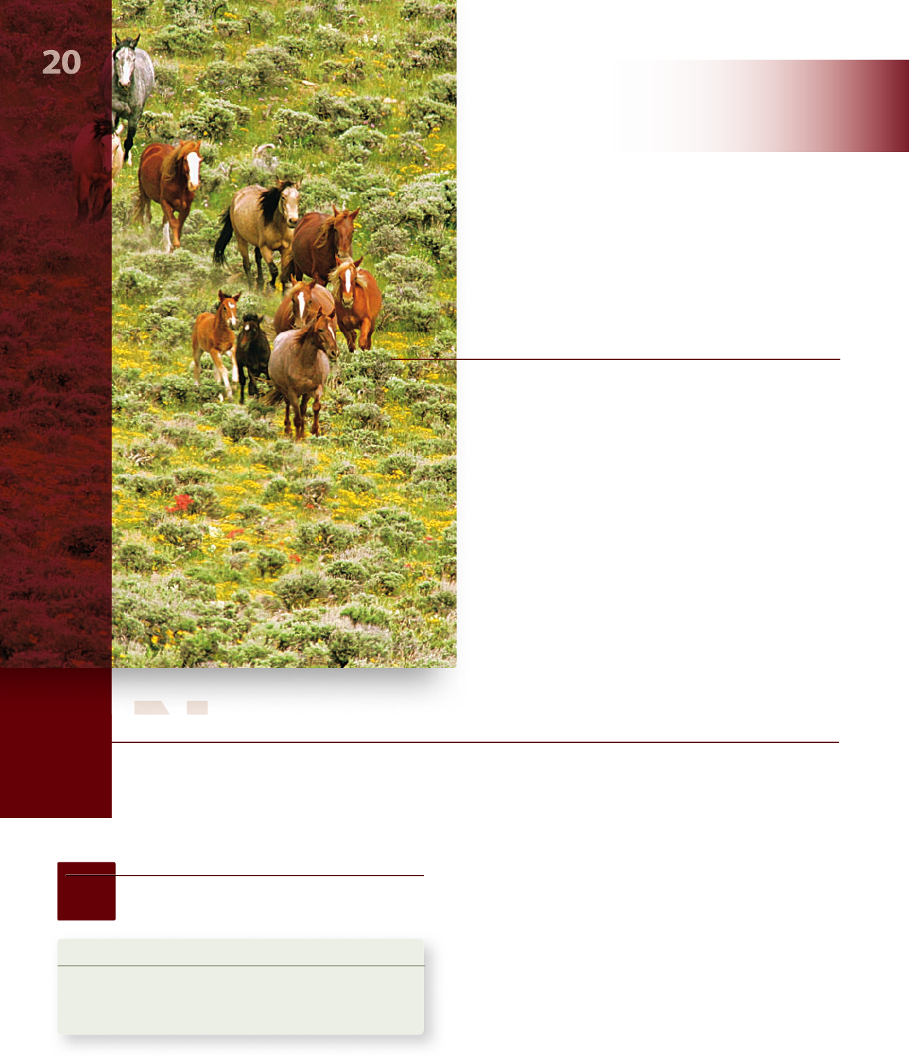
Chapter
20
Genes Within
Populations
Introduction
No other human being is exactly like you (unless you have an identical twin). Often the particular characteristics of an
individual have an important bearing on its survival, on its chances to reproduce, and on the success of its offspring.
Evolution is driven by such factors, as different alleles rise and fall in populations. These dece ptively simple matters lie at the
core of evolutionary biology, which is the topic of this chapter and chapters 21 through 25.
Genetic variation, that is, differences in alleles of genes found
within individuals of a population, provides the raw material for
natural selection, which will be described shortly. Natural pop-
ulations contain a wealth of such variation. In plants, insects,
and vertebrates, many genes exhibit some level of variation. In
this chapter, we explore genetic variation in natural populations
and consider the evolutionary forces that cause allele frequen-
cies in natural populations to change.
The word evolution is widely used in the natural and social
sciences. It refers to how an entity—be it a social system, a gas,
20.1
Genetic Variation and Evolution
Learning Outcomes
Define 1. evolution and population genetics.
Explain the difference between evolution by natural 2.
selection and the inheritance of acquired characteristics.
CHAPTER
Part
IV
Evolution
rav32223_ch20_396-416.indd 396rav32223_ch20_396-416.indd 396 11/10/09 4:26:12 PM11/10/09 4:26:12 PM
Apago PDF Enhancer
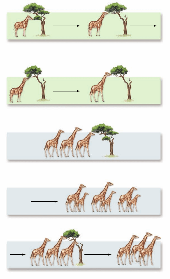
a. Lamarck’s theory: acquired variation is passed on to descendants.
b. Darwin’s theory: natural selection or genetically-based variation leads to
evolutionary change.
Reproduction
Reproduction
Reproduction
Natural
selection
Stretching Stretching
The giraffe ancestor lengthened its
neck by stretching to reach tree leaves,
then passed the change to offspring.
Some individuals born happen to have longer necks due to
genetic differences.
Individuals pass on their traits to next generation.
Proposed ancestor of
giraffes has characteristics
of modern-day okapi.
Over many generations, longer-necked individuals are more successful,
perhaps because they can feed on taller trees, and pass the long-neck
trait on to their offspring.
x x
Figure 20.1
Two ideas of how gira es might have
evolved long necks.
or a planet—changes through time. Although development of
the modern concept of evolution in biology can be traced to
Darwin’s landmark work, On the Origin of Species, the first five
editions of his book never actually used the term. Rather, Dar-
win used the phrase “descent with modification.”
Although many more complicated definitions have
been proposed, Darwin’s words probably best capture the es-
sence of biological evolution: Through time, species accu-
mulate differences; as a result, descendants differ from their
ancestors. In this way, new species arise from existing ones.
Many processes can lead
to evolutionary change
You have already learned about the development of Darwin’s
ideas in chapter 1 . Darwin was not the first to propose a theory
of evolution. Rather, he followed a long line of earlier philoso-
phers and naturalists who deduced that the many kinds of or-
ganisms around us were produced by a process of evolution.
Unlike his predecessors, however, Darwin proposed
natural selection as the mechanism of evolution. Natural selec-
tion produces evolutionary change when some individuals in a
population possess certain inherited characteristics and then
produce more surviving offspring than individuals lacking these
characteristics. As a result, the population gradually comes to
include more and more individuals with the advantageous char-
acteristics. In this way, the population evolves and becomes bet-
ter adapted to its local circumstances.
A rival theory, championed by the prominent biologist
Jean-Baptiste Lamarck, was that evolution occurred by the
inheritance of acquired characteristics. According to La-
marck, changes that individuals acquired during their lives
were passed on to their offspring. For example, Lamarck pro-
posed that ancestral giraffes with short necks tended to stretch
their necks to feed on tree leaves, and this extension of the
neck was passed on to subsequent generations, leading to the
long-necked giraffe (figure 20.1a). In Darwin’s theory, by con-
trast, the variation is not created by experience, but is the re-
sult of preexisting genetic differences among individuals
(figure 20.1b).
One way to monitor how populations change through
time is to look at changes in the frequencies of alleles of a gene
from one generation to the next. Natural selection, by favoring
individuals with certain alleles, can lead to change in such allele
frequencies, but it is not the only process that can do so. Allele
frequencies can also change when mutations occur repeatedly,
changing one allele to another, and when migrants bring alleles
into a population. In addition, when populations are small, the
frequencies of alleles can change randomly as the result of
chance events. Often, natural selection overwhelms the effects
of these other processes, but as you will see later in this chapter,
this is not always the case.
Evolution can result from any process that causes a
change in the genetic composition of a population. We can-
not talk about evolution, therefore, without also consider-
ing population genetics, the study of the properties of
genes in populations.
Populations contain ample genetic variation
It is best to start by looking at the genetic variation present
among individuals within a species. This is the raw material
available for the selective process.
As you saw in chapter 12 , a natural population can con-
tain a great deal of genetic variation. How much variation usu-
ally occurs? Humans are representative of most—but not
all—species in that human populations contain substantial
amounts of genetic variation. For example:
Genes that in uence blood groups. 1. Chemical analysis
has revealed the existence of more than 30 blood group
genes in humans, in addition to the ABO locus. At least
chapter
20
Genes Within Populations
397www.ravenbiology.com
rav32223_ch20_396-416.indd 397rav32223_ch20_396-416.indd 397 11/10/09 4:26:17 PM11/10/09 4:26:17 PM
Apago PDF Enhancer
one third of these genes are routinely found in several
alternative allelic forms in human populations. In addition
to these, more than 45 variable genes encode other
proteins in human blood cells and plasma that are not
considered blood groups. In short, many genetically
variable genes are present in this one system alone.
Genes that in uence enzymes.2. Alternative alleles of
genes specifying particular enzymes are easy to
distinguish by measuring how fast the alternative proteins
migrate in an electrical eld (a process called electrophoresis—
see chapter 17 ). A great deal of variation exists at enzyme-
specifying loci. About 5% of the enzyme loci of a typical
human are heterozygous: If you picked an individual at
random, and in turn selected one of the enzyme-encoding
genes of that individual at random, the chances are 1 in 20
(5%) that the gene you selected would be heterozygous in
that individual.
Considering the entire genome, it is fair to say that all
humans are different from one another except for identical
twins. This is also true of other organisms, except for those that
reproduce asexually. In nature, genetic variation is the rule.
Enzyme polymorphism
Many loci in a particular population have more than one allele at
frequencies significantly greater than would occur due to muta-
tion alone. Researchers refer to such a locus as polymorphic
(figure 20.2). The extent of such variation within natural popula-
tions was not even suspected a few decades ago, when modern
techniques such as protein electrophoresis made it possible to
examine enzymes and other proteins directly.
We now know that most populations of insects and plants
are polymorphic at more than half of their enzyme-encoding
loci, that is, the loci have more than one allele occurring at a
frequency greater than 5%. Vertebrates are somewhat less poly-
morphic. Heterozygosity, the probability that a randomly se-
lected gene will be heterozygous in a randomly selected
individual, is about 15% in Drosophila and other invertebrates,
between 5% and 8% in vertebrates, and around 8% in out-
crossing plants (values of heterozygosity tend to be lower than
the proportion of loci that are polymorphic because for loci
that are polymorphic, many individuals within the population
will be homozygous). These high levels of genetic variability
provide ample supplies of raw material for evolution.
DNA sequence polymorphism
The advent of gene technology has made it possible to assess
genetic variation even more directly by sequencing the DNA
itself. For example, when the ADH genes (which encode for
alcohol dehydrogenase) of 11 Drosophila melanogaster individu-
als were sequenced, scientists found 43 variable sites, only 1 of
which had been detected by protein electrophoresis.
Numerous other studies of variation at the DNA level
have confirmed these findings: Abundant variation exists in
both the coding regions of genes and in their nontranslated
introns—considerably more variation than we can detect by ex-
amining enzymes with electrophoresis.
Learning Outcomes Review 20.1
Evolution can be described as descent with modifi cation. Natural selection
occurs when individuals carrying certain alleles leave more off spring
than those without the alleles. Natural populations contain more genetic
variation than can be accounted for by mutation alone. Population genetics
studies this variability through statistical analyses.
■ Why is genetic variation in a population necessary for
evolution to occur?
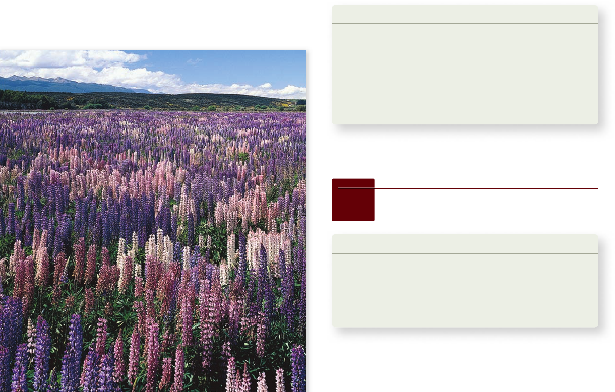
Figure 20.2
Polymorphic variation. This natural
population of loosestrife, Lythrum salicaria, exhibits considerable
variation in ower color. Individual differences are inherited and
passed on to offspring.
20.2
Changes in Allele Frequency
Learning Outcomes
Explain the Hardy–Weinberg principle.1.
Describe the characteristics of a population that is in 2.
Hardy–Weinberg equilibrium.
Demonstrate how the operation of evolutionary 3.
processes can be detected.
rav32223_ch20_396-416.indd 398rav32223_ch20_396-416.indd 398 11/10/09 4:26:17 PM11/10/09 4:26:17 PM

Apago PDF Enhancer
Generation One Generation Two
Phenotypes
Genotypes BB Bb bb
0.36 0.48
84% 16%
0.16
0.36 + 0.24 = 0.60B 0.24 + 0.16 = 0.40b
Frequency of
genotype in population
Frequency of gametes
Eggs
bb
q
2
= 0.16
Bb
pq = 0.24
Bb
pq = 0.24
p
2
+2pq+q
2
= 1
BB
p
2
= 0.36
b
q = 0.40
B
p = 0.60
b
q = 0.40
B
p = 0.60
Sperm
The Hardy–Weinberg equation with two alleles:
A binomial expansion
In algebraic terms, the Hardy–Weinberg principle is written as
an equation. Consider a population of 100 cats in which 84 are
black and 16 are white. The frequencies of the two phenotypes
would be 0.84 (or 84%) black and 0.16 (or 16%) white. Based
on these phenotypic frequencies, can we deduce the underlying
frequency of genotypes?
If we assume that the white cats are homozygous reces-
sive for an allele we designate as b, and the black cats are either
homozygous dominant BB or heterozygous Bb, we can calcu-
late the allele frequencies of the two alleles in the population
from the proportion of black and white individuals, assuming
that the population is in Hardy–Weinberg equilibrium.
Let the letter p designate the frequency of the B allele and
the letter q the frequency of the alternative allele. Because there
are only two alleles, p plus q must always equal 1 (that is, the
total population). In addition, we know that the sum of the
three genotype frequencies must also equal 1. If the frequency
of the B allele is p, then the probability that an individual will
have two B alleles is simply the probability that each of its al-
leles is a B. The probability of two events happening indepen-
dently is the product of the probability of each event; in this
case, the probability that the individual received a B allele from
its father is p, and the probability the individual received a B
allele from its mother is also p, so the probability that both hap-
pened is p * p = p
2
(figure 20.3). By the same reasoning, the prob-
ability that an individual will have two b alleles is q
2
.
What about the probability that an individual will be a
heterozygote? There are two ways this could happen: The indi-
vidual could receive a B from its father and a b from its mother,
or vice versa. The probability of the first case is p * q and the
probability of the second case is q * p. Because the result in ei-
ther case is that the individual is a heterozygote, the probability
of that outcome is the sum of the two probabilities, or 2pq.
Genetic variation within natural populations was a puzzle to Dar-
win and his contemporaries in the mid-1800s. The way in which
meiosis produces genetic segregation among the progeny of a hy-
brid had not yet been discovered. And, although Mendel per-
formed his experiments during this same time period, his work
was largely unknown. Selection, scientists then thought, should
always favor an optimal form, and so tend to eliminate variation.
Moreover, the theory of blending inheritance—in which offspring
were expected to be phenotypically intermediate relative to their
parents—was widely accepted. If blending inheritance were cor-
rect, then the effect of any new genetic variant would quickly be
diluted to the point of disappearance in subsequent generations.
The Hardy–Weinberg principle allows
prediction of genotype frequencies
Following the rediscovery of Mendel’s research, two people in
1908 solved the puzzle of why genetic variation persists—
Godfrey H. Hardy, an English mathematician, and Wilhelm
Weinberg, a German physician. These workers were initially
confused about why, after many generations, a population didn’t
come to be composed solely of individuals with the dominant
phenotype. The conclusion they independently came to was
that the original proportions of the genotypes in a population
will remain constant from generation to generation, as long as
the following assumptions are met:
No mutation takes place.1.
No genes are transferred to or from other sources (no 2.
immigration or emigration takes place).
Random mating is occurring.3.
The population size is very large.4.
No selection occurs.5.
Because the genotypes’ proportions do not change, they
are said to be in Hardy–Weinberg equilibrium.
Inquiry question
?
If all white cats died, what proportion of the kittens in the next generation would be white?
Figure 20.3
The Hardy–Weinberg equilibrium. In the absence of factors that alter them, the frequencies of gametes, genotypes, and
phenotypes remain constant generation after generation.
chapter
20
Genes Within Populations
399www.ravenbiology.com
rav32223_ch20_396-416.indd 399rav32223_ch20_396-416.indd 399 11/10/09 4:26:20 PM11/10/09 4:26:20 PM
Apago PDF Enhancer
So, to summarize, if a population is in Hardy–Weinberg
equilibrium with allele frequencies of p and q, then the prob-
ability that an individual will have each of the three possible
genotypes is p
2
+ 2pq + q
2
. You may recognize this as the bino-
mial expansion:
(p + q)
2
= p
2
+ 2pq + q
2
Finally, we may use these probabilities to predict the dis-
tribution of genotypes in the population, again assuming that
the population is in Hardy–Weinberg equilibrium. If the prob-
ability that any individual is a heterozygote is 2pq, then we
would expect the proportion of heterozygous individuals in the
population to be 2pq; similarly, the frequency of BB and bb ho-
mozygotes would be expected to be p
2
and q
2
.
Let us return to our example. Remember that 16% of the
cats are white. If white is a recessive trait, then this means that
such individuals must have the genotype bb. If the frequency of
this genotype is q
2
= 0.16 (the frequency of white cats), then q
(the frequency of the b allele) = 0.4. Because p + q = 1, therefore,
p, the frequency of allele B, would be 1.0 – 0.4 = 0.6 (remember,
the frequencies must add up to 1). We can now easily calculate
the expected genotype frequencies: homozygous dominant
BB cats would make up the p
2
group, and the value of p
2
= (0.6)
2
= 0.36, or 36 homozygous dominant BB individuals in a popula-
tion of 100 cats. The heterozygous cats have the Bb genotype
and would have the frequency corresponding to 2pq, or (2 * 0.6
*
0.4) = 0.48, or 48 heterozygous Bb individuals.
Using the Hardy–Weinberg equation to predict
frequencies in subsequent generations
The Hardy–Weinberg equation is another way of expressing the
Punnett square described in chapter 12, with two alleles assigned
frequencies, p and q. Figure 20.3 allows you to trace genetic re-
assortment during sexual reproduction and see how it affects the
frequencies of the B and b alleles during the next generation.
In constructing this diagram, we have assumed that the
union of sperm and egg in these cats is random, so that all com-
binations of b and B alleles occur. The alleles are therefore
mixed randomly and are represented in the next generation in
proportion to their original occurrence. Each individual egg or
sperm in each generation has a 0.6 chance of receiving a B allele
( p = 0.6) and a 0.4 chance of receiving a b allele (q = 0.4).
In the next generation, therefore, the chance of combining
two B alleles is p
2
, or 0.36 (that is, 0.6 * 0.6), and approximately
36% of the individuals in the population will continue to have
the BB genotype. The frequency of bb individuals is q
2
(0.4 * 0.4)
and so will continue to be about 16%, and the frequency of Bb
individuals will be 2pq (2 * 0.6 * 0.4), or on average, 48%.
Phenotypically, if the population size remains at 100 cats,
we would still see approximately 84 black individuals (with either
BB or Bb genotypes) and 16 white individuals (with the bb geno-
type). Allele, genotype, and phenotype frequencies have remained
unchanged from one generation to the next, despite the reshuf-
fling of genes that occurs during meiosis and sexual reproduc-
tion. Dominance and recessiveness of alleles can therefore be
seen only to affect how an allele is expressed in an individual and
not how allele frequencies will change through time.
Hardy–Weinberg predictions can be
applied to data to nd evidence
of evolutionary processes
The lesson from the example of black and white cats is that if
all five of the assumptions listed earlier hold true, the allele and
genotype frequencies will not change from one generation to
the next. But in reality, most populations in nature will not fit
all five assumptions. The primary utility of this method is to
determine whether some evolutionary process or processes are
operating in a population and, if so, to suggest hypotheses about
what they may be.
Suppose, for example, that the observed frequencies of
the BB, bb, and Bb genotypes in a different population of cats
were 0.6, 0.2, and 0.2, respectively. We can calculate the allele
frequencies for B as follows: 60% (0.6) of the cats have two B
alleles, 20% have one, and 20% have none. This means that the
average number of B alleles per cat is 1.4 [(0.6 × 2) + (0.2 × 1) +
(0.2 × 0) = 1.4
]. Because each cat has two alleles for this gene, the
frequency is 1.4/2.0 = 0.7. Similarly, you should be able to cal-
culate that the frequency of the b allele = 0.3.
If the population were in Hardy–Weinberg equilibrium,
then, according to the equation earlier in this section, the fre-
quency of the BB genotype would be 0.7
2
= 0.49, lower than it
really is. Similarly, you can calculate that there are fewer
heterozygotes and more bb homozygotes than expected; then
clearly, the population is not in Hardy–Weinberg equilibrium.
What could cause such an excess of homozygotes and
deficit of heterozygotes? A number of possibilities exist, includ-
ing (1) natural selection favoring homozygotes over heterozy-
gotes, (2) individuals choosing to mate with genetically similar
individuals (because BB * BB and bb * bb matings always produce
homozygous offspring, but only half of Bb * Bb produce hetero-
zygous offspring, such mating patterns would lead to an excess
of homozygotes), or (3) an influx of homozygous individuals
from outside populations (or conversely, emigration of hetero-
zygotes to other populations). By detecting a lack of Hardy–
Weinberg equilibrium, we can generate potential hypotheses
that we can then investigate directly.
The operation of evolutionary processes can be detected
in a second way. As discussed previously, if all of the Hardy–
Weinberg assumptions are met, then allele frequencies will stay
the same from one generation to the next. Changes in allele
frequencies between generations would indicate that one of the
assumptions is not met.
Suppose, for example, that the frequency of b was 0.53 in
one generation and 0.61 in the next. Again, there are a number
of possible explanations: For example, (1) selection favoring in-
dividuals with b over B, (2) immigration of b into the population
or emigration of B out of the population, or (3) high rates of
mutation that more commonly occur from B to b than vice ver-
sa. Another possibility is that the population is a small one, and
that the change represents the random fluctuations that result
because, simply by chance, some individuals pass on more of
their genes than others. We will discuss how each of these pro-
cesses is studied in the rest of the chapter.
400
part
IV
Evolution
rav32223_ch20_396-416.indd 400rav32223_ch20_396-416.indd 400 11/10/09 4:26:21 PM11/10/09 4:26:21 PM

Apago PDF Enhancer
Mutagen DNA
T
A
G
G
G
G
C
C
Self-fertilization
a. The ultimate source of
variation. Individual
mutations occur so rarely
that mutation alone usually
does not change allele
frequency much.
b. A very potent agent of
change. Individuals or
gametes move from one
population to another.
c. Inbreeding is the most
common form. It does not
alter allele frequency but
reduces the proportion of
heterozygotes.
d. Statistical accidents. The
random fluctuation in allele
frequencies increases as
population size decreases.
e. The only agent that
produces adaptive
evolutionary changes.
Mutation Gene Flow Nonrandom Mating Genetic Drift Selection
20.3
Five Agents of Evolutionary
Change
Learning Outcomes
Define the five processes that can cause evolutionary 1.
change.
Explain how these processes can cause populations to 2.
deviate from Hardy-Weinberg Equilibrium
The five assumptions of the Hardy–Weinberg principle also
indicate the five agents that can lead to evolutionary change in
populations. They are mutation, gene flow, nonrandom mating,
genetic drift in small populations, and the pressures of natural
selection. Any one of these may bring about changes in allele or
genotype proportions.
Learning Outcomes Review 20.2
The Hardy–Weinberg principle states that in a large population with
no selection and random mating, the proportion of alleles does not
change through the generations. Finding that a population is not in
Hardy–Weinberg equilibrium indicates that one or more evolutionary
agents are operating.
■ If you know the genotype frequencies in a population,
how can you determine whether the population is in
Hardy–Weinberg equilibrium?
Mutation changes alleles
Mutation from one allele to another can obviously change the
proportions of particular alleles in a population. Mutation rates
are generally so low that they have little effect on the Hardy–
Weinberg proportions of common alleles. A typical gene mu-
tates about once per 100,000 cell divisions. Because this rate is
so low, other evolutionary processes are usually more impor-
tant in determining how allele frequencies change.
Nonetheless, mutation is the ultimate source of genetic
variation and thus makes evolution possible (figure 20.4a). It is
important to remember, however, that the likelihood of a par-
ticular mutation occurring is not affected by natural selection;
that is, mutations do not occur more frequently in situations in
which they would be favored by natural selection.
Gene ow occurs when alleles move
between populations
Gene flow is the movement of alleles from one population to
another. It can be a powerful agent of change. Sometimes gene
flow is obvious, as when an animal physically moves from one
place to another. If the characteristics of the newly arrived indi-
vidual differ from those of the animals already there, and if the
newcomer is adapted well enough to the new area to survive
and mate successfully, the genetic composition of the receiving
population may be altered.
Other important kinds of gene flow are not as obvious.
These subtler movements include the drifting of gametes or
the immature stages of plants or marine animals from one place
to another (figure 20.4b). Pollen, the male gamete of flowering
plants, is often carried great distances by insects and other ani-
mals that visit flowers. Seeds may also blow in the wind or be
carried by animals to new populations far from their place of
Figure 20.4
Five agents o f evolutionary change. a. Mutation, (b) gene ow, (c) nonrandom mating, (d) genetic drift, and
(e) selection.
chapter
20
Genes Within Populations
401www.ravenbiology.com
rav32223_ch20_396-416.indd 401rav32223_ch20_396-416.indd 401 11/10/09 4:26:21 PM11/10/09 4:26:21 PM