Schmuller J. Statistical Analysis with Excel For Dummies

Подождите немного. Документ загружается.

219

Chapter 12: Testing More Than Two Samples

In fact, it’s .14, which is way beyond acceptable. (The mathematics behind

calculating that number is a little involved, so I won’t elaborate.)

With more than three samples, the situation gets even worse. Four groups

require six t-tests, and the probability that at least one of them is significant

is .26. Table 12-2 shows what happens with increasing numbers of samples.

Table 12-2 The Incredible Increasing Alpha

Number of Samples t Number of Tests Pr(At Least One Significant t)

.14

.26

.40

.54

.66

.76

.84

.90

Carrying out multiple t-tests is clearly not the answer. So what do you do?

A solution

It’s necessary to take a different approach. The idea is to think in terms of

variances rather than means.

I’d like you to think of variance in a slightly different way. The formula for

estimating population variance, remember, is

Because the variance is almost a mean of squared deviations from the mean,

statisticians also refer to it as Mean Square. In a way, that’s an unfortunate

nickname: It leaves out “deviation from the mean,” but there you have it.

18 454060-ch12.indd 21918 454060-ch12.indd 219 4/21/09 7:31:34 PM4/21/09 7:31:34 PM

220

Part III: Drawing Conclusions from Data

The numerator of the variance, excuse me, Mean Square, is the sum of

squared deviations from the mean. This leads to another nickname, Sum of

Squares. The denominator, as I say in Chapter 10, is degrees of freedom (df).

So, the slightly different way to think of variance is

You can abbreviate this as

Now, on to solving the thorny problem. One important step is to find the

Mean Squares hiding in the data. Another is to understand that you use these

Mean Squares to estimate the variances of the populations that produced

these samples. In this case, assume those variances are equal, so you’re

really estimating one variance. The final step is to understand that you use

these estimates to test the hypotheses I show you at the beginning of the

chapter.

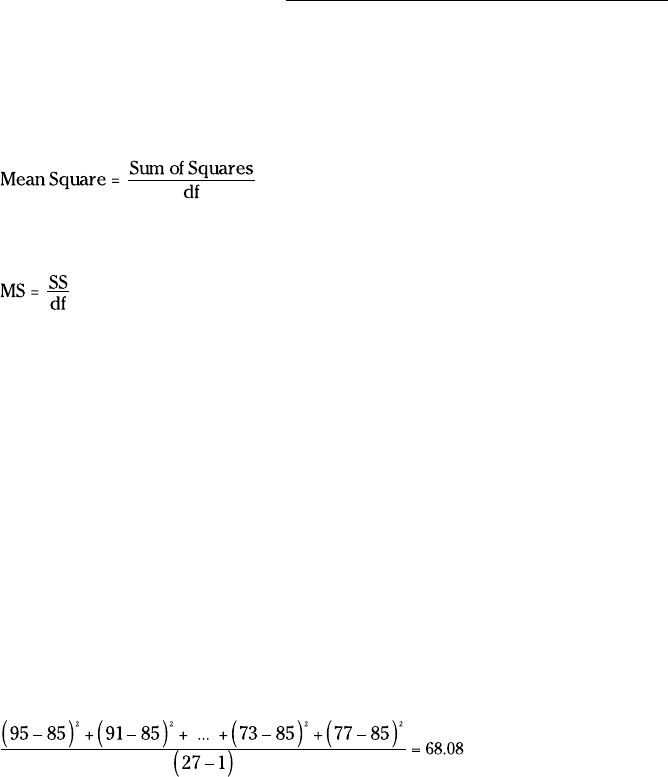
Three different Mean Squares are inside the data in Table 12-1. Start with the

whole set of 27 scores, forgetting for the moment that they’re divided into

three groups. Suppose you want to use those 27 scores to calculate an esti-

mate of the population variance. (A dicey idea, but humor me.) The mean of

those 27 scores is 85. I’ll call that mean the grand mean because it’s the aver-

age of everything.

So the Mean Square would be

The denominator has 26 (27–1) degrees of freedom. I refer to that variance

as the Total Variance, or in the new way of thinking about this, the MS

Total

. It’s

often abbreviated as MS

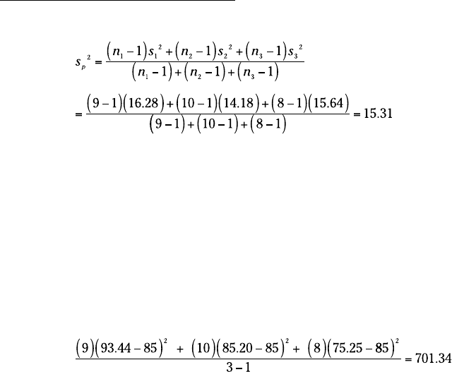
Here’s another variance to consider. In Chapter 11, I describe the t-test for

two samples with equal variances. For that test, you put the two sample

variances together to create a pooled estimate of the population variance.

The data in Table 12-1 provide three sample variances for a pooled estimate:

16.28, 14.18, 15.64. Assuming these numbers represent equal population vari-

ances, the pooled estimate is:

18 454060-ch12.indd 22018 454060-ch12.indd 220 4/21/09 7:31:35 PM4/21/09 7:31:35 PM

221

Chapter 12: Testing More Than Two Samples

Because this pooled estimate comes from the variance within the groups, it’s

called MS

Within

, or MS

One more Mean Square to go — the variance of the sample means around

the grand mean. In this example, that means the variance in these numbers:

93.44, 85.20, and 75.25 — sort of. I said “sort of” because these are means,

not scores. When you deal with means you have to take into account the

number of scores that produced each mean. To do that you multiply each

squared deviation by the number of scores in that sample.

So this variance is:

The df for this variance is 2 (the number of samples – 1).

Statisticians, not known for their crispness of usage, refer to this as the vari-

ance between sample means. (Among is the correct word when you’re talking

about more than two items.) This variance is known as MS

Between

, or MS

So you now have three estimates of population variance: MS

, MS

, and MS

What do you do with them?

Remember that the original objective is to test a hypothesis about three

means. According to H

, any differences you see among the three sample

means are due strictly to chance. The implication is that the variance among

those means is the same as the variance of any three numbers selected at

random from the population.

If you could somehow compare the variance among the means (that’s MS

remember) with the population variance, you could see if that holds up. If

only you had an estimate of the population variance that’s independent of

the differences among the groups, you’d be in business.

Ah . . . but you do have that estimate. You have MS

, an estimate based on

pooling the variances within the samples. Assuming those variances repre-

sent equal population variances, this is a pretty solid estimate. In this exam-

ple, it’s based on 24 degrees of freedom.

18 454060-ch12.indd 22118 454060-ch12.indd 221 4/21/09 7:31:35 PM4/21/09 7:31:35 PM

222

Part III: Drawing Conclusions from Data

The reasoning now becomes: If MS

is about the same as MS

, you have evi-

dence consistent with H

. If MS

is significantly larger than MS

, you have evi-

dence that’s inconsistent with H

. In effect, you transform these hypotheses

: μ

= μ

: Not H

into these

: σ

≤ σ

: σ

> σ

Rather than multiple t-tests among sample means, you perform a test of the

difference between two variances.

What is that test? In Chapter 11 I show you the test for hypotheses about

two variances. It’s called the F-test. To perform this test, you divide one vari-

ance by the other. You evaluate the result against a family of distributions

called the F-distribution. Because two variances are involved, two values for

degrees of freedom define each member of the family.

For this example, F has df = 2 (for the MS

) and df = 24 (for the MS

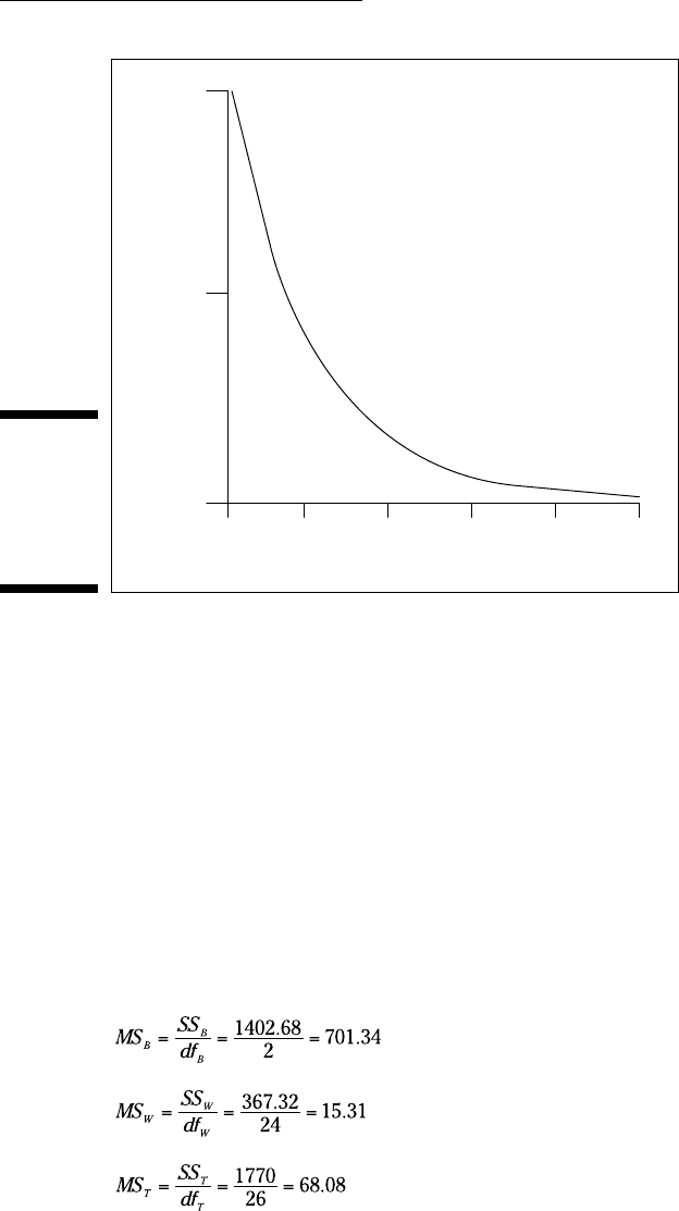
Figure 12-1 shows what this member of the F family looks like. For our

purposes, it’s the distribution of possible F values if H

is true.

The test statistic for the example is:

What proportion of area does this value cut off in the upper tail of the

F-distribution? From Figure 12-1, you can see that this proportion is micro-

scopic, as the values on the horizontal axis only go up to 5. (And the propor-

tion of area beyond 5 is tiny.) It’s way less than .05.

This means that it’s highly unlikely that differences among the means are due

to chance. It means that you reject H

This whole procedure for testing more than two samples is called the analysis

of variance, often abbreviated as ANOVA. In the context of an ANOVA, the

denominator of an F-ratio has the generic name error term. The independent

variable is sometimes called a factor. So this is a single-factor or (one-factor)

ANOVA.

18 454060-ch12.indd 22218 454060-ch12.indd 222 4/21/09 7:31:35 PM4/21/09 7:31:35 PM

223

Chapter 12: Testing More Than Two Samples

Figure 12-1:

The

F-distribution

with 2 and

24 degrees

of freedom.

012345

0.0

0.5

1.0

f(F)

In this example, the factor is Training Method. Each instance of the indepen-

dent variable is called a level. The independent variable in this example has

three levels.

More complex studies have more than one factor, and each factor can have

many levels.

Meaningful relationships

Take another look at the Mean Squares in this example, each with its Sum of

Squares and degrees of freedom. Before, when I calculated each Mean Square

for you, I didn’t explicitly show you each Sum of Squares, but here I include

them:

18 454060-ch12.indd 22318 454060-ch12.indd 223 4/21/09 7:31:35 PM4/21/09 7:31:35 PM

224

Part III: Drawing Conclusions from Data

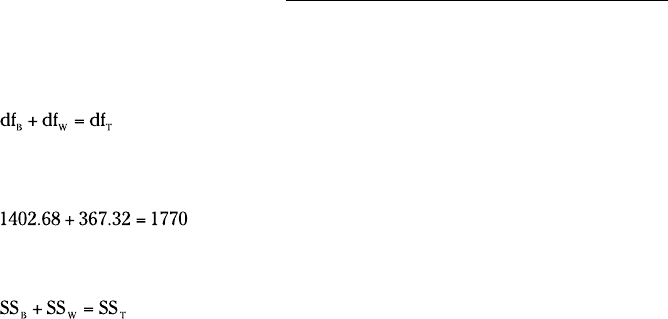
Start with the degrees of freedom: df

= 2, df

= 24, and df

= 26. Is it a coinci-

dence that they add up? Hardly. It’s always the case that

How about those Sums of Squares?

Again, this is no coincidence. In the analysis of variance, this always happens:

In fact, statisticians who work with the analysis of variance speak of parti-

tioning (read “breaking down into non-overlapping pieces”) the SS

into one

portion for the SS

and another for the SS

, and partitioning the df

into one

amount for the df

and another for the df

After the F-test

The F-test enables you to decide whether or not to reject H

. After you decide

to reject, then what? All you can say is that somewhere within the set of

means, something is different from something else. The F-test doesn’t specify

what those “somethings” are.

Planned comparisons

In order to get more specific, you have to do some further tests. Not only

that, you have to plan those tests in advance of carrying out the ANOVA.

What are those tests? Given what I said earlier, this might surprise you:

t-tests. While this might sound inconsistent with the increased alpha of mul-

tiple t-tests, it’s not. If an analysis of variance enables you to reject H

, then

it’s OK to use t-tests to turn the magnifying glass on the data and find out

where the differences are. And as I’m about to show you, the t-test you use is

slightly different from the one I discuss in Chapter 11.

These post-ANOVA t-tests are called planned comparisons. Some refer to

them as a priori tests. I illustrate by following through with the example.

Suppose before you gathered the data, you had reason to believe that

Method 1 would result in higher scores than Method 2, and that Method

2 would result in higher scores than Method 3. In that case, you plan in

advance to compare the means of those samples in the event your ANOVA-

based decision is to reject H

18 454060-ch12.indd 22418 454060-ch12.indd 224 4/21/09 7:31:35 PM4/21/09 7:31:35 PM

225

Chapter 12: Testing More Than Two Samples

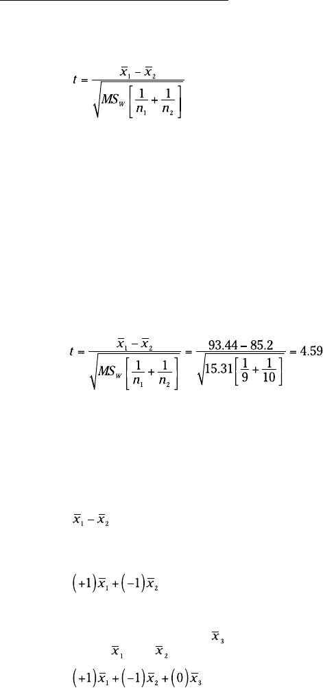
The formula for this kind of t-test is

It’s a test of

: μ

≤ μ

: μ

> μ

takes the place of the pooled estimate s

I show you in Chapter 11. In

fact, when I introduced MS

, I showed how it’s just a pooled estimate that

can incorporate variances from more than two samples. The df for this t-test

is df

, rather than (n

– 1) + (n

– 1).

For this example, the Method 1 versus Method 2 comparison is:

With df = 24, this value of t cuts off a miniscule portion of area in the upper

tail of the t-distribution. The decision is to reject H

The planned comparison t-test formula I showed you matches up with the

t-test for two samples. You can write the planned comparison t-test formula

in a way that sets up additional possibilities. Start by writing the numerator

a bit differently:

The +1 and –1 are comparison coefficients. I refer to them, in a general way, as

and c

. In fact, c

and can enter the comparison, even if you’re just com-

paring

with :

The important thing is that the coefficients add up to zero.

18 454060-ch12.indd 22518 454060-ch12.indd 225 4/21/09 7:31:36 PM4/21/09 7:31:36 PM

226

Part III: Drawing Conclusions from Data

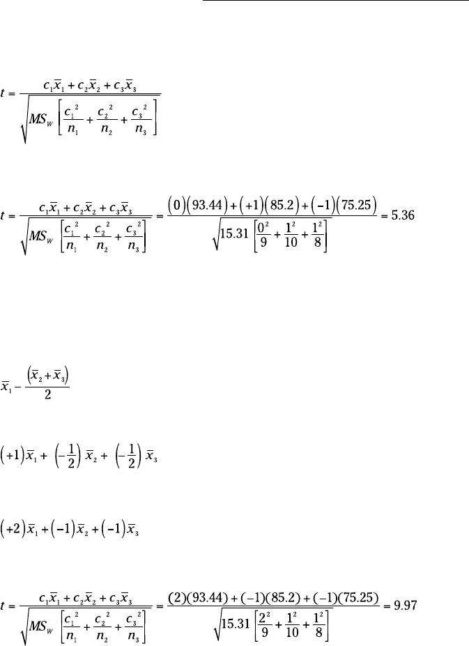
Here’s how the comparison coefficients figure into the planned comparison

t-test formula for a study that involves three samples:

Applying this formula to Method 2 versus Method 3:

The value for t indicates the results from Method 2 are significantly higher

than the results from Method 3.

You can also plan a more complex comparison — say, Method 1 versus the

average of Method 2 and Method 3. Begin with the numerator. That would be

With comparison coefficients, you can write this as

If you’re more comfortable with whole numbers, you can write it as:

Plugging these whole numbers into the formula gives you

Again, strong evidence for rejecting H

18 454060-ch12.indd 22618 454060-ch12.indd 226 4/21/09 7:31:36 PM4/21/09 7:31:36 PM

227

Chapter 12: Testing More Than Two Samples

Unplanned comparisons

Things would get boring if your post-ANOVA testing is limited to compari-

sons you have to plan in advance. Sometimes you want to snoop around

your data and see if anything interesting reveals itself. Sometimes something

jumps out at you that you didn’t anticipate.

When this happens, you can make comparisons you didn’t plan on. These

comparisons are called a posteriori tests, post hoc tests, or simply unplanned

comparisons. Statisticians have come up with a wide variety of these tests,

many of them with exotic names and many of them dependent on special

sampling distributions.

The idea behind these tests is that you pay a price for not having planned

them in advance. That price has to do with stacking the deck against reject-

ing H

for the particular comparison.

Of all the unplanned tests available, the one I like best is a creation of famed

statistician Henry Scheffé. As opposed to esoteric formulas and distributions,

you start with the test I already showed you, and then add a couple of easy-

to-do extras.

The first extra is to understand the relationship between t and F. I’ve shown

you the F-test for three samples. You can also carry out an F-test for two

samples. That F-test has df = 1 and df = (n

– 1) + (n

– 1). The df for the t-test,

of course, is (n

– 1) + (n

– 1). Hmmm . . . seems like they should be related

somehow.

They are. The relationship between the two-sample t and the two-sample F is

Now I can tell you the steps for performing Scheffé’s test:

1. Calculate the planned comparison t-test.

2. Square the value to create F.

3. Find the critical value of F for dfB and dfW at α = .05 (or whatever α

you choose).

4. Multiply this critical F by the number of samples – 1.

The result is your critical F for the unplanned comparison. I’ll call this F’.

5. Compare the calculated F to F’. If the calculated F is greater, reject H0

for this test. If it’s not, don’t reject H0 for this test.

18 454060-ch12.indd 22718 454060-ch12.indd 227 4/21/09 7:31:36 PM4/21/09 7:31:36 PM

228

Part III: Drawing Conclusions from Data

Imagine that in the example, you didn’t plan in advance to compare the mean

of Method 1 with the mean of Method 3. (In a study involving only three sam-

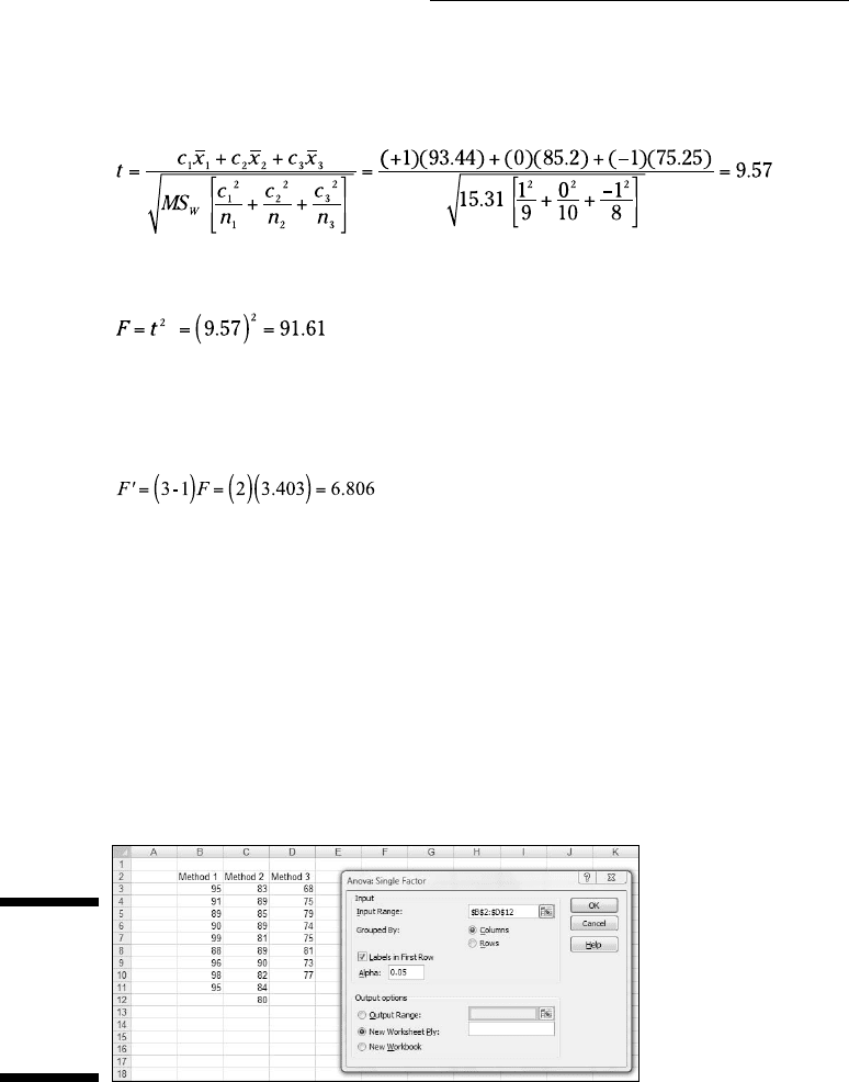
ples that’s hard to imagine, I grant you.) The t-test is:

Squaring this result gives

For F with 2 and 24 df and α = .05, the critical value is 3.403. (You can look

that up in a table in a statistics textbook or you can use the worksheet func-

tion FINV.) So

Because the calculated F, 91.61, is greater than F’, the decision is to reject

. You have evidence that Method 1’s results are different from Method 3’s

results.

Data analysis tool: Anova: Single Factor

The calculations for the ANOVA can get intense. Excel has a data analysis

tool that does the heavy lifting. It’s called Anova: Single Factor. Figure 12-2

shows this tool along with the data for the preceding example.

Figure 12-2:

The Anova:

Single

Factor data

analysis tool

dialog box.

18 454060-ch12.indd 22818 454060-ch12.indd 228 4/21/09 7:31:37 PM4/21/09 7:31:37 PM