Schmuller J. Statistical Analysis with Excel For Dummies

Подождите немного. Документ загружается.

339

Chapter 17: More on Probability

The upper limit is:

1. Select a cell for BETAINV’s answer.

2. From the Statistical Functions menu, select BETAINV to open its

Function Arguments dialog box (Figure 17-3).

Figure 17-3:

The

BETAINV

Function

Arguments

dialog box.

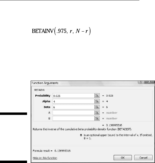
3. In the Function Arguments dialog box, enter the appropriate values

for the arguments.

The X box holds a cumulative probability. For the lower bound of the 95

percent confidence limits, the probability is .025.

In the Alpha box, I entered the number of successes. For this example

that’s 4.

In the Beta box, I entered the number of failures (NOT the number of

trials). The number of failures is 6.

The A box and the B box are evaluation limits for the value in the X box.

Again, these aren’t relevant for this type of example. I left them blank,

which by default sets A = 0 and B=1.

With the entries for X, Alpha, and Beta, the answer appears in the dialog

box. The answer for this example is .13699536.

4. Click OK to put the answer into the selected cell.

Entering .975 in the X box gives .700704575 as the result. So the 95 percent

confidence limits for the probability of a success are .137 and .701 (rounded

off) if you have 4 successes in 10 trials.

24 454060-ch17.indd 33924 454060-ch17.indd 339 4/21/09 7:36:42 PM4/21/09 7:36:42 PM

340

Part IV: Working with Probability

With more trials of course, the confidence limit narrows. For 40 successes in

100 trials, the confidence limits are .307 and .497

Poisson

If you have the kind of process that produces a binomial distribution, and

you have an extremely large number of trials and a very small number of suc-

cesses, the Poisson distribution approximates the binomial. The equation of

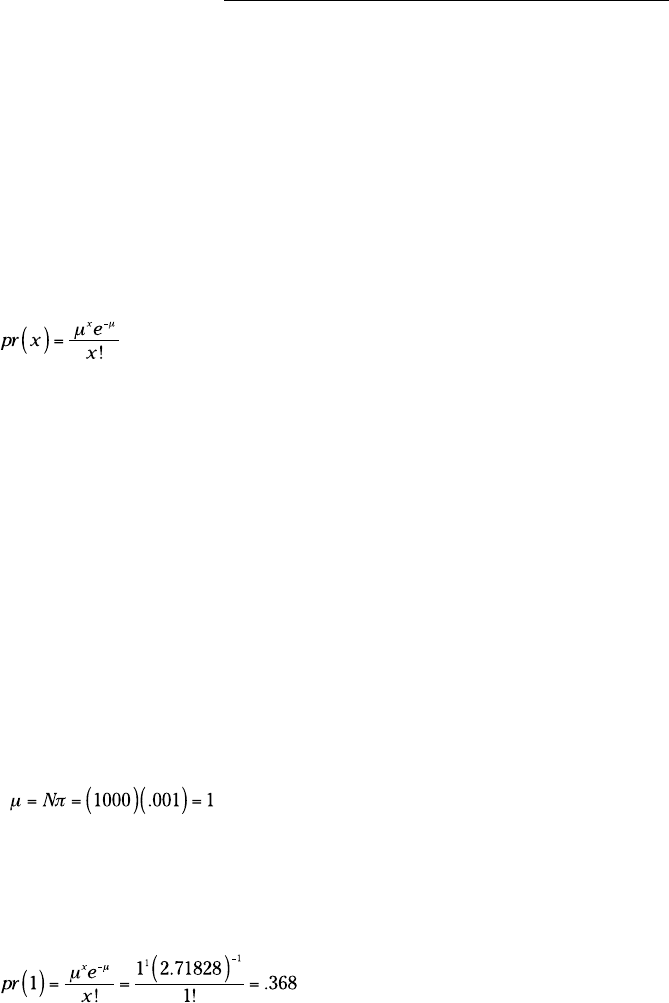
the Poisson is

In the numerator, μ is the mean number of successes in the trials, and e is

2.71828 (and infinitely more decimal places), a constant near and dear to the

hearts of mathematicians.

Here’s an example. The FarKlempt Robotics Inc. produces a universal joint

for its robots’ elbows. The production process is under strict computer con-

trol, so that the probability a joint is defective is .001. What is the probability

that in a sample of 1000, one joint is defective? What’s the probability that

two are defective? Three?

Named after 19th-century mathematician Siméon-Denis Poisson, this distribu-

tion is computationally easier than the binomial — or at least it was when

mathematicians had no computational aids. With Excel, you can easily use

BINOMDIST to do the binomial calculations.

First, I apply the Poisson distribution to the FarKlempt example. If π = .001

and N = 1000, the mean is

(See Chapter 16 for an explanation of μ = N π .)

Now for the Poisson. The probability that one joint in a sample of 1000 is

defective is:

24 454060-ch17.indd 34024 454060-ch17.indd 340 4/21/09 7:36:43 PM4/21/09 7:36:43 PM

341

Chapter 17: More on Probability

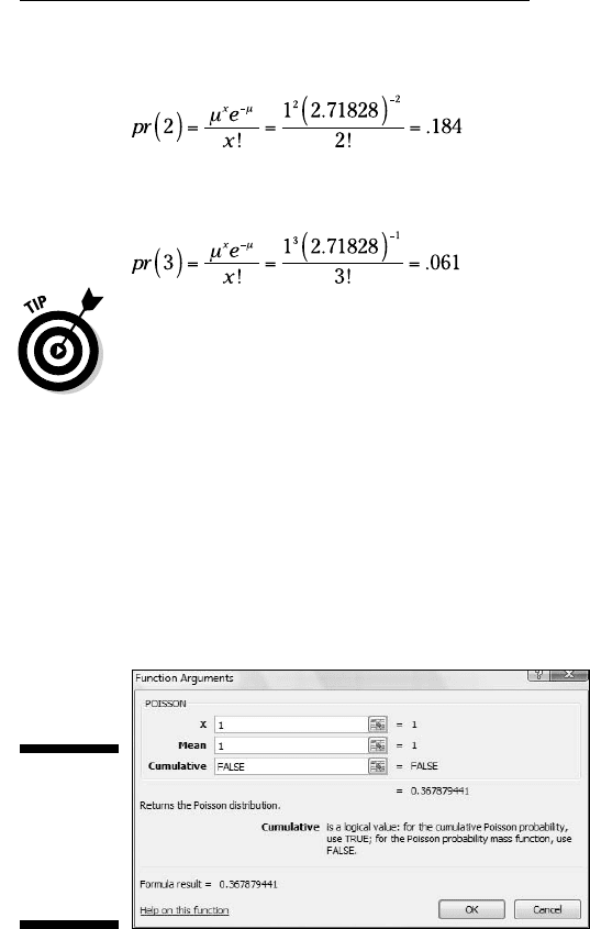
For two defective joints in 1000, it’s

And for three defective joints in 1000:

As you read through this, it may seem odd that I refer to a defective item as a

“success.” Remember, that’s just a way of labeling a specific event.

POISSON

Here are the steps for using Excel’s POISSON for the preceding example:

1. Select a cell for POISSON’s answer.

2. From the Statistical Functions menu, select POISSON to open its

Function Arguments dialog box (Figure 17-4).

Figure 17-4:

The

POISSON

Function

Arguments

dialog box.

3. In the Function Arguments dialog box, enter the appropriate values

for the arguments.

In the X box, I entered the number of events for which I’m determining

the probability. I’m looking for pr(1), so I entered 1.

. In the Mean box, I entered the mean of the process. That’s N π, which for

this example is 1.

24 454060-ch17.indd 34124 454060-ch17.indd 341 4/21/09 7:36:43 PM4/21/09 7:36:43 PM

342

Part IV: Working with Probability

In the Cumulative box, it’s either TRUE for the cumulative probability or

FALSE for just the probability of the number of events. I entered FALSE.

. With the entries for X, Mean, and Cumulative, the answer appears in the

dialog box. The answer for this example is .367879441.

4. Click OK to put the answer into the selected cell.

In the example, I showed you the probability for two defective joints in 1,000

and the probability for three. To follow through with the calculations, I’d

type 2 into the X box to calculate pr(2), and 3 to find pr(3).

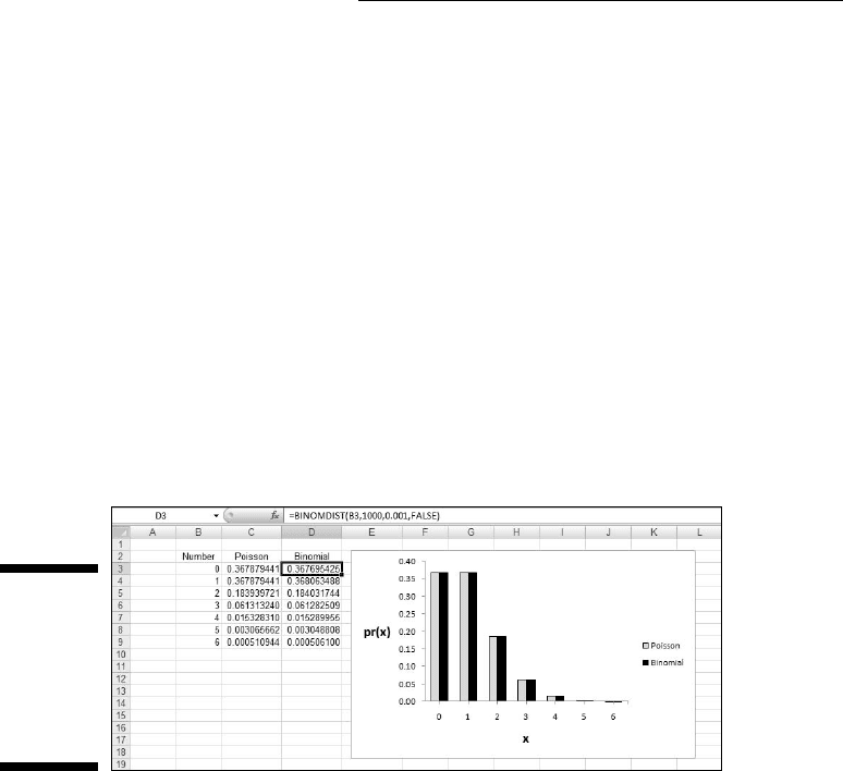
As I said before, in the 21st century, it’s pretty easy to calculate the binomial

probabilities directly. Figure 17-5 shows you the Poisson and the Binomial

probabilities for the numbers in Column B and the conditions of the example.

I graphed the probabilities so you can see how close the two really are. I

selected Cell D3 so the formula box shows you how I used BINOMDIST to cal-

culate the binomial probabilities.

Figure 17-5:

Poisson

prob-

abilities and

Binomial

probabili-

ties.

Although the Poisson’s usefulness as an approximation is outdated, it has

taken on a life of its own. Phenomena as widely disparate as reaction time

data in psychology experiments, degeneration of radioactive substances, and

scores in professional hockey games seem to fit Poisson distributions. This is

why business analysts and scientific researchers like to base models on this

distribution. (“Base models on?” What does that mean? I tell you all about it

in Chapter 18.)

Gamma

The gamma distribution is related to the Poisson distribution in the same way

the negative binomial distribution is related to the binomial. The negative

24 454060-ch17.indd 34224 454060-ch17.indd 342 4/21/09 7:36:43 PM4/21/09 7:36:43 PM

343

Chapter 17: More on Probability

binomial tells you the number of trials until a specified number of successes

in a binomial distribution. The gamma distribution tells you how many sam-

ples you go through to find a specified number of successes in a Poisson dis-

tribution. Each sample can be a set of objects (as in the FarKlempt Robotics

universal joint example), a physical area, or a time interval.

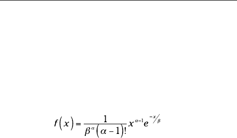
The probability density function for the gamma distribution is:

Again, this works when α is a whole number. If it’s not, you guessed it —

calculus. (By the way, when this function has only whole-number values of

α it’s called the Erlang distribution, just in case anybody ever asks you.) The

letter e, once again, is the constant 2.7818 I told you about earlier.

Don’t worry about the exotic-looking math. As long as you understand what

each symbol means, you’re in business. Excel does the heavy lifting for you.

So here’s what the symbols mean. For the FarKlempt Robotics example, α is

the number of successes and β corresponds to μ the Poisson distribution.

The variable x tracks the number of samples. So if x is 3, α is 2, and β is 1,

you’re talking about the probability density associated with finding the second

success in the third sample, if the average number of successes per sample

(of 1000) is 1. (Where does 1 come from, again? That’s 1000 universal joints

per sample multiplied by .001, the probability of producing a defective one.)

To determine probability, you have to work with area under the density func-

tion. This brings me to the Excel worksheet function designed for gamma.

GAMMADIST

GAMMADIST gives you a couple of options. You can use it to calculate the

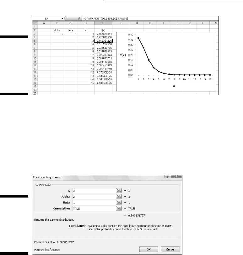
probability density, and you can use it to calculate probability. Figure 17-6

shows how I used the first option to create a graph of the probability density

so you can see what the function looks like. Working within the context of the

example I just laid out, I set Alpha to 2, Beta to 1, and calculated the density

for the values of x in Column D.

The values in Column E shows the probability densities associated with find-

ing the second defective universal joint in the indicated number of samples

of 1000. For example, Cell E5 holds the probability density for finding the

second defective joint in the third sample.

24 454060-ch17.indd 34324 454060-ch17.indd 343 4/21/09 7:36:43 PM4/21/09 7:36:43 PM

344

Part IV: Working with Probability

Figure 17-6:

The density

function

for gamma,

with

Alpha = 2

and Beta =1.

In real life, you work with probabilities rather than densities. Next, I show

you how to use GAMMADIST to determine the probability of finding the

second defective joint in the third sample. Here it is:

1. Select a cell for GAMMADIST’s answer.

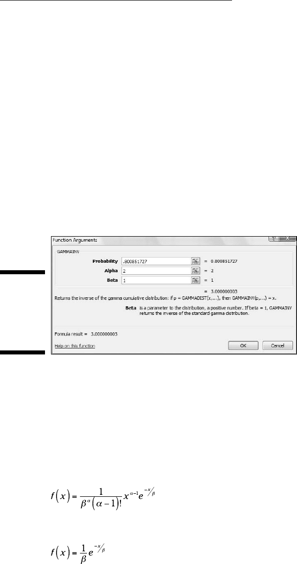
2. From the Statistical Functions menu, select GAMMADIST to open its

Function Arguments dialog box (Figure 17-7).

Figure 17-7:

The

GAMMA

DIST

Function

Arguments

dialog box.

3. In the Function Arguments dialog box, enter the appropriate values

for the arguments.

The X box holds the number of samples for which I’m determining the

probability. I’m looking for pr(3), so I entered 3.

In the Alpha box, I entered the number of successes. I want to find the

second success in the third sample, so I entered 2.

In the Beta box, I entered the average number of successes that occur

within a sample. For this example, that’s 1.

In the Cumulative box the choices are TRUE for the cumulative distribu-

tion or FALSE to find the probability density. I want to find the probabil-

ity, not the density, so I entered TRUE.

24 454060-ch17.indd 34424 454060-ch17.indd 344 4/21/09 7:36:43 PM4/21/09 7:36:43 PM

345

Chapter 17: More on Probability

With values entered for X, Alpha, Beta, and Cumulative, the answer —

.800851727 — appears in the dialog box.

4. Click OK to put the answer into the selected cell.

GAMMAINV

If you want to know, at a certain level of probability, how many samples it

takes to observe a specified number of successes, this is the function for you.

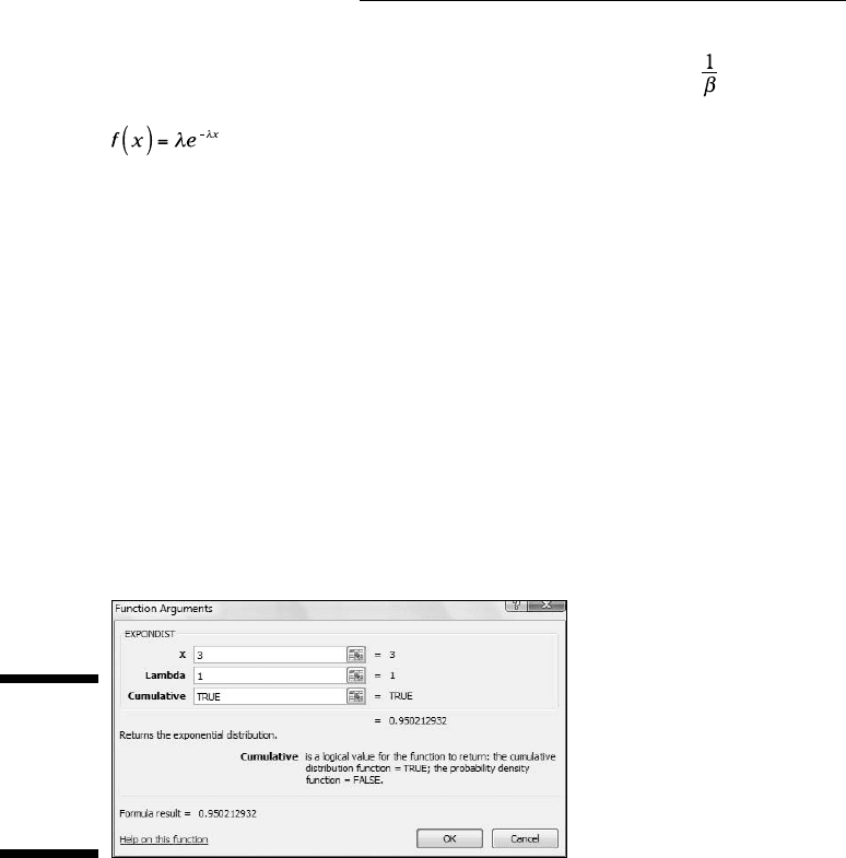
GAMMAINV is the inverse of GAMMADIST. Enter a probability along with

Alpha and Beta and it returns the number of samples. Its Function Arguments

dialog box has a Probability box, an Alpha box, and a Beta box. Figure

17-8 shows that if you enter the answer for the preceding section into the

Probability box and the same numbers for Alpha and Beta, the answer is 3.

(Well, actually, a tiny bit more than 3.)

Figure 17-8:

The

GAMMAINV

Function

Arguments

dialog box.

Exponential

If you’re dealing with the gamma distribution and you have Alpha = 1, you

have the exponential distribution. This gives the probability that it takes a

specified number of samples to get to the first success.

What does the density function look like? Excuse me . . . I’m about to go mathemat-

ical on you for a moment. Here, once again, is the density function for gamma:

If α = 1, it looks like this:

24 454060-ch17.indd 34524 454060-ch17.indd 345 4/21/09 7:36:44 PM4/21/09 7:36:44 PM

346

Part IV: Working with Probability

Statisticians like substituting λ (the Greek letter “lambda”) for , so here’s

the final version:

I bring this up because Excel’s EXPONDIST Function Arguments dialog box

has a box for LAMBDA, and I want you to know what it means.

EXPONDIST

Use EXPONDIST to determine the probability that it takes a specified number

of samples to get to the first success in a Poisson distribution. Here, I work

once again with the universal joint example. I show you how to find the prob-

ability that you’ll see the first success in the third sample.

1. Select a cell for EXPONDIST’s answer.

2. From the Statistical Functions menu, select EXPONDIST to open its

Function Arguments dialog box (Figure 17-9).

Figure 17-9:

The

EXPONDIST

Function

Arguments

dialog box.

3. In the Function Arguments dialog box, enter the appropriate values

for the arguments.

In the X box, I entered the number of samples for which I’m determining

the probability. I’m looking for pr(3), so I typed 3.

In the Lambda box, I entered the average number of successes per

sample. This goes back to the numbers I gave you in the example — the

probability of a success (.001) times the number of universal joints in

each sample (1000). That product is 1, so I entered 1 in this box.

24 454060-ch17.indd 34624 454060-ch17.indd 346 4/21/09 7:36:44 PM4/21/09 7:36:44 PM

347

Chapter 17: More on Probability

In the Cumulative box, the choices are TRUE for the cumulative distribu-

tion or FALSE to find the probability density. I want to find the probabil-

ity, not the density, so I entered TRUE.

With values entered for X, Lambda, and Cumulative, the answer appears

in the dialog box. The answer for this example is .950212932.

4. Click OK to put the answer into the selected cell.

24 454060-ch17.indd 34724 454060-ch17.indd 347 4/21/09 7:36:44 PM4/21/09 7:36:44 PM

348

Part IV: Working with Probability

24 454060-ch17.indd 34824 454060-ch17.indd 348 4/21/09 7:36:44 PM4/21/09 7:36:44 PM