Schneider P., Eberly D.H. Geometric Tools for Computer Graphics
Подождите немного. Документ загружается.

514 Chapter 11 Intersection in 3D
C
r
h
â
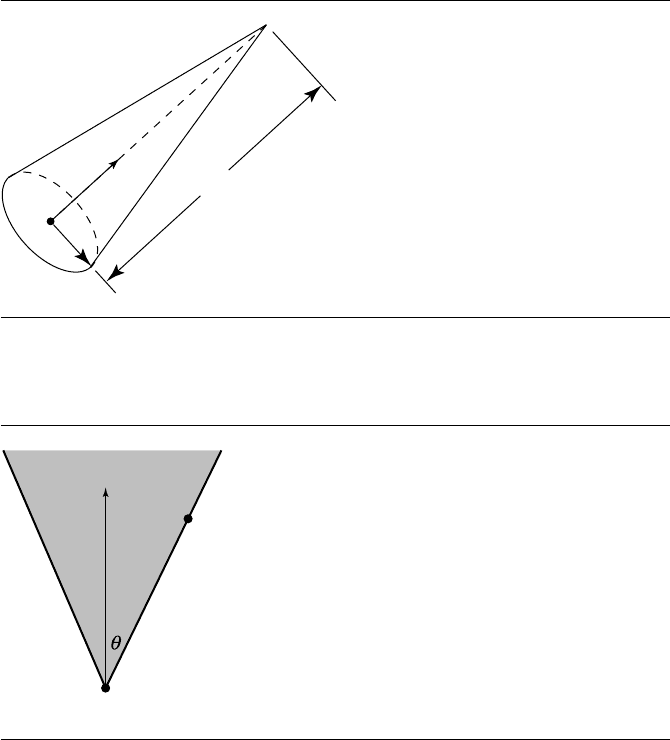
Figure 11.14
General cone representation.
V
X
â
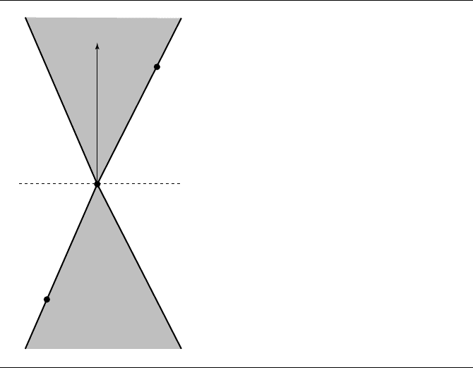
Figure 11.15 An acute cone. The inside region is shaded.
Figure 11.15 shows a 2D representation of the cone. The shaded portion indicates
the inside of the cone, a region represented algebraically by replacing = in the above
equation with ≥.
To avoid the square root calculation X − V , the cone equation may be squared
to obtain the quadratic equation
ˆa ·(X − V)
2
= (cos
2
θ)X − V
2
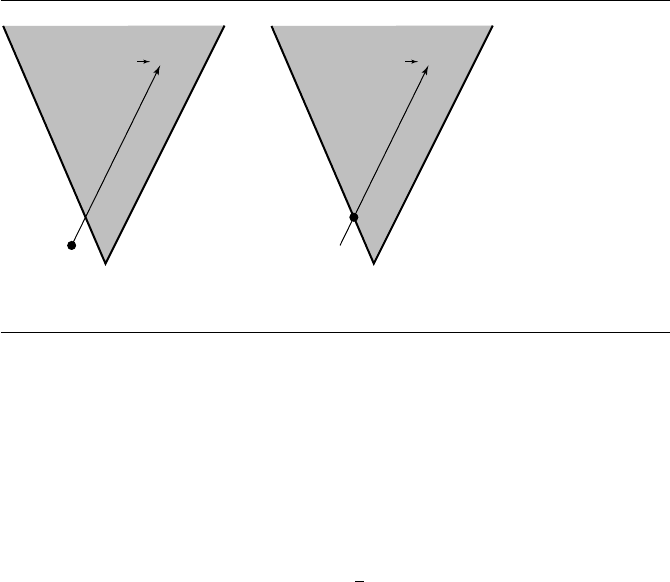
However, the set of points satisfying this equation is a double cone. The original cone
is on the side of the plane ˆa · (X −V)=0 to which ˆa points. The quadratic equation
11.3 Linear Components and Quadric Surfaces 515
V
X
â
2V – X
Figure 11.16 An acute double cone. The inside region is shaded.
defines the original cone and its reflection through the plane. Specifically, if X is a
solution to the quadratic equation, then its reflection through the vertex, 2V − X,is
also a solution. Figure 11.16 shows the double cone. To eliminate the reflected cone,
any solutions to the quadratic equation must also satisfy ˆa · (X −V)≥ 0. Also, the
quadratic equation can be written as a quadratic form, (X − V)
T
M(X − V)= 0,
where M = ( ˆa ˆa
T
− γ
2
I) and γ = cos θ . Therefore, X is a point on the acute cone
whenever
(X − V)
T
M(X − V)= 0 and ˆa ·(X − V)≥0
To find the intersection points of the line and the cone, replace X(t) in the
quadratic equation and simplify to obtain c
2
t
2
+ 2c
1
t + c
0
= 0, where
= P − V ,
c
2
=
d
T
M
d, c
1
=
d
T
M
, and c
0
=
T
M
. The following discussion analyzes the
quadratic equation to determine points of intersection of the line with the double
cone. The dot product test to eliminate points on the reflected cone must be applied
to these points.
It is possible that the quadratic equation is degenerate in the sense that c
2
= 0.
In this case the equation is linear, but even that might be degenerate in the sense
516 Chapter 11 Intersection in 3D
P
d
P
d
(a) (b)
Figure 11.17 Case c
2
= 0. (a) c
0
= 0; (b) c
0
= 0.
that c
1
= 0. An implementation must take this into account when finding the inter-
sections.
First, suppose that c
2
= 0. Define δ = c
2
1
− c
0
c
2
.Ifδ<0, then the quadratic
equation has no real-valued roots, in which case the line does not intersect the double
cone. If δ = 0, then the equation has a repeated real-valued root t =−c
1
/c
2
, in which
case the line is tangent to the double cone at a single point. If δ>0, the equation has
two distinct real-valued roots t = (−c
1
±
√
δ)/c
2
, in which case the line penetrates
the double cone at two points.
Second, suppose that c
2
= 0. This means
d
T
M
d = 0. A consequence is that the
line V + s
d is on the double cone for all s ∈ R. Geometrically, the line P + t
d
is parallel to some line on the cone. If additionally c
0
= 0, this condition implies
T
M
= 0. A consequence is that P is a point on the double cone. Even so, it is
not necessary that the original line is completely contained by the cone (although it
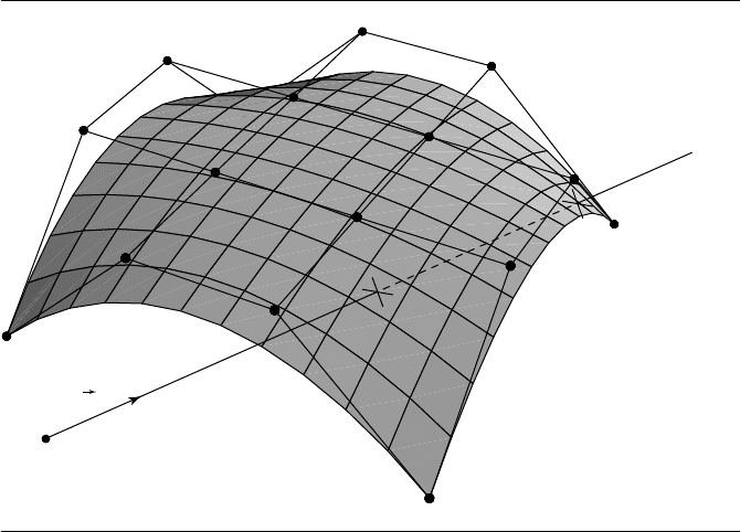
is possible that it is). Figure 11.17 shows the cases c
2
=0 and c
0
=0orc
0
=0. Finally,
if c
i
=0 for all i, then P + t
d is on the double cone for all t ∈R. Algebraically, when
c
1
= 0, the root to the linear equation is t =−c
2
/(2c
1
).Ifc
1
= 0 and c
2
= 0, the line
does not intersect the cone. If c
1
= c
2
= 0, then the line is contained by the double
cone.
The pseudocode is
bool LineConeIntersection(Line3D line, Cone3D cone, Point3D closestIntesection)
{
Vector3D axis = cone.axis;
float cosTheta = cos(cone.theta);
Matrix4x4 M = axis * axis.transpose() - cosTheta * cosTheta * Matrix4x4::Identity;
11.3 Linear Components and Quadric Surfaces 517
float c2, c1, c0, discrm;
Vec3D delta = line.origin - cone.vertex;
c2 = line.direction.transpose()*M*line.direction;
c1 = line.direction.transpose()*M*delta;
c0 = delta.transpose()*M*delta;
discrm = c1 * c1 - c2 * c0;
if (discrm > 0) {
float t[3];
Point3D ipoint[3];
int minIndex;
bool valid[3];
if (fabs(c2) < zeroEpislon) {
if (fabs(c1) < zeroEpislon) {
valid[0] = false;
valid[1] = false;
} else {
t[0] = -c0 / (2 * c1);
ipoint[0] = line.origin + t[0] * line.direction;
}
} else {
t[0] = (-c2 + sqrt(discrm)) / c0;
t[1] = (-c2 - sqrt(discrm)) / c0;
ipoint[0] = line.origin + t[0] * line.direction;
ipoint[1] = line.origin + t[1] * line.direction;
float scalarProjection;
if (scalarProjection = Dot(axis,ipoint[0] - cone.vertex) < 0) {
valid[0] = false;
} else {
if (scalarProjection > cone.height) {
valid[0] = false;
} else {
valid[0] = true;
}
}
if (scalarProjection = Dot(axis,ipoint[1] - cone.vertex) < 0) {
valid[1] = false;
518 Chapter 11 Intersection in 3D
} else {
if (scalarProjection > cone.height) {
valid[1] = false;
} else {
valid[1] = true;
}
}
}
// Check for earlier intersection with cap
Plane3D p1;
p1.normal = axis;
p1.origin = cone.vertex + cone.height * axis;
if (lineIntersectPlane(p1, line, t[3])) {
ipoint[3] = line.origin + t[3] * line.direction;
if (distance(p1.origin, ipoint[3]) <= cone.radius) {
valid[3] = true;
} else {
valid[3] = false;
}
} else {
valid[3] = false;
}
// Now find earliest valid intersection
bool hit = false;
int minIndex = 0;
float mint = infinity;
for(i=0;i<3;i++) {
if (valid[i]) {
if (t[i] < mint) {
mint = t[i];
minIndex = i;
hit = true;
}
}
}
closestIntersection = ipoint[minIndex];
return hit;
} else if (discrm == 0) {
// No need to check cap
float scalarProjection;

11.4 Linear Components and Polynomial Surfaces 519
t[0] = -c1 / c2;
ipoint[0] = line.origin + t[0] * line.direction;
if (scalarProjection = dotProd(axis, ipoint[0] - cone.vertex) >= 0) {
if (scalarProjection <= cone.height) {
closestIntersection = ipoint[0];
return true;
}
}
}
return false;
}
11.4 Linear Components and Polynomial
Surfaces
A polynomial surface is a vector-valued function X : D ⊂ R
2
→ R
3
,say,X(s, t),
whose domain is D and range is R. The components X
i
(s, t) of X(s, t) areeacha
polynomial in the specified parameters
X
i
(s, t) =
n
i
j=0
m
i
k=0
a
ij k
s
j
t
k
(11.14)
where n
i
+ m
i
is the degree of the polynomial. The domain D is typically either R
2
or [0, 1]
2
.Arational polynomial surface is a vector-valued function X(s, t) whose
components X
i
(s, t) are ratios of polynomials
X
i
(s, t) =
n
i
j=0
m
i
k=0
a
ij k
s
j
t
k
p
i
j=0
q
i
k=0
b
ij k
s
j
t
k
where n
i
+m
i
is the degree of the numerator polynomial and p
i
+q
i
is the degree of
the denominator polynomial.
A few common types of surfaces that occur in computer graphics are B
´
ezier
surfaces, B-spline surfaces, and nonuniform rational B-spline (NURBS) surfaces.
For the purposes of the following discussion, a linear component is defined in the
usual fashion as an origin plus a direction vector
L(t) = P + t
d (11.15)
where −∞≤ t ≤∞for a line, 0 ≤ t ≤∞for a ray, and for a segment {P
0
, P
1
} we
have
d = P
1
− P
0
and 0 ≤t ≤ 1.
520 Chapter 11 Intersection in 3D
P
d
Figure 11.18 Intersection of a ray with a NURBS surface.
The two most common situations requiring the intersection of a polynomial
surface and a linear component are in rendering—specifically, ray tracing—and in
interactive applications in the process of selection or picking, in which the user uses a
mouse or other pointing device to specify an object. In light of this observation, we’ll
concentrate on ray-surface intersection. An example is shown in Figure 11.18.
11.4.1 Algebraic Surfaces
Algebraic surfaces are those defined, in general, by an equation of the form
f(x, y, z) = 0 (11.16)
where the function f is a polynomial; that is,
f(x, y, z) =
l
i=0
m
j=0
n
k=0
a
ij k
x
i
y
j
z
k
whose degree is the sum of the degrees of the components: d = l +m + n.
11.4 Linear Components and Polynomial Surfaces 521
If we rewrite Equation 11.15 in its component form
x =P
x
+ td
x
y =P
y
+ td
y
z = P
z
+ td
z
it can easily be seen that if we substitute this into Equation 11.16, we get another
polynomial equation, of the form
g(t) =
d
i=0
a
i
t
i
which can be solved using a standard method. Note that the maximum number of
real roots of this equation is the same as the degree of the polynomial surface. In fact,
for equations of degree four or less, easy analytic solutions are available. For higher-
order equations, a numerical approach is necessary; Hanrahan (1983) used a method
for first isolating the roots (Collins and Akritas 1976; Collins and Loos 1982), and
then applied regula falsi.
11.4.2 Free-Form Surfaces
A free-form parametric surface is defined in general as shown in Equation 11.14.
The intersection of a linear component with a polynomial Cartesian product patch
is a polynomial equation of degree 2 × M
2
,whereM is the degree of the surface;
for a bicubic patch, this means we get a polynomial intersection equation of degree
18. Taking a direct root-finding approach (such as Newton iteration) can result in a
very slow algorithm that may fail to converge in some cases. In any case, predictable
behavior results only when the initial guess is reasonably near the first root.
Kajiya (1982) presented an approach that has been adopted by later researchers
and is worth outlining: a ray can be considered to be the intersection of two (nonpar-
allel) planes. To intersect a ray with a patch, the surface equation is substituted into
the plane equations; this gives us two equations defining the algebraic curves formed
by the intersection of the patch with the two planes. The intersection of these two
curves gives the (u, v) parameters of the point at which the ray intersects the patch.
Kajiya then used Laguerre’s method for root finding in order to solve the equations;
he finds it superior to Newton’s method in stability and the property that it con-
verges on the nearest root irrespective of the original guess, and that it is cubically
convergent. Others have also exploited this approach of considering the ray as the in-
tersection of two planes (Sweeney and Bartels 1986; Martin et al. 2000). A full proof
of the validity of this approach is found in Kajiya (1982).
522 Chapter 11 Intersection in 3D
P
d
Figure 11.19 Failed intersection calculation due to insufficient surface tessellation (shown in cross
section for clarity).
An alternative approach is to simply subdivide or tessellate the surface into poly-
gons (either triangles or quads, typically), and then intersect the ray with each of these
tessellants. This is very simple to program, but has several problems:
It can be extremely inefficient if some sort of spatial-partitioning scheme is also
not employed (e.g., bounding volume hierarchy).
If the subdivision is not sufficiently fine, then there is a good chance that an
intersection will be missed (see Figure 11.19).
If the subdivision is too fine, then more (expensive) computation has been done
than is necessary, but accuracy increases with subdivision granularity, and so
there is an inherent incompatibility of goals.
Broadly stated, the direct evaluation approach can be quite slow, but very accurate,
while the simple subdivision approach can be efficient, but may sacrifice accuracy
while achieving that efficiency. Naturally, you may think of creating a hybrid of the
two approaches, and this has, indeed, been done with good results.
Before describing these hybrid approaches, a few other interesting methods are
worth mentioning. Nishita, Sederberg, and Kakimoto (1990) describe an approach
they call “B
´
ezier clipping”; the ray is considered to be the intersection of two orthog-
onal planes, and the B
´
ezier surface is projected onto a plane perpendicular to the ray.
The ray then is projected to a point, and the two planes are projected to two per-
pendicular lines; this forms an orthonormal basis. Distances between the (projected)
control points and the “basis vectors” are computed, and the patch is “clipped” by
11.4 Linear Components and Polynomial Surfaces 523
use of the de Casteljau algorithm—portions of the surface that could not possibly
contain the intersection are no longer considered. Once the size of the successively
clipped patch reaches a specified size threshhold, the intersection is computed to be
the center of the sufficiently small patch.
Fournier and Buchanan (1984) describe a method in which Chebyshev polyno-
mials are used both to represent the polynomial surface and to create tight bounding
boxes. The patch is approximated by adaptively subdividing it into a large number
of bilinear patches. These bilinear patches are organized into a bounding box hier-
archy to speed up ray intersections. The bounding box hierarchy is traversed to the
leaf node intersecting the ray, and the intersection of the ray with the bilinear patch
at that leaf is used as the (approximate) intersection of the ray with the surface.
Both of these methods were analyzed by Campagna, Slusallek, and Seidel (1997).
Their results show what you might expect—the B
´
ezier clipping approach was rela-
tively slower than the Chebyshev boxing method (25–30%). They also noted that the
Chebyshev boxing approach can only handle integral patches. As a result of these
analyses, they developed their own bounding volume hierarchy approach that could
handle rational patches and that was of comparable speed to the Chebyshev boxing
approach.
Toth (1985) describes a ray intersection algorithm that is also based on Kajiya’s
approach; it also uses Newton iteration, but solves the problem of providing a good
initial guess by the use of interval analysis techniques.
The general structure of the algorithm we’ll present here has been utilized by
Martin et al. (2000), Sweeney and Bartels (1986), and Campagna, Slusallek, and
Seidel (1997). They all share a few basic ideas, which we’ll now address.
Intersecting a Ray and a Parametric Polynomial Surface
Polynomial surfaces may be represented in your choice of basis. Here, we use the
B
´
ezier basis because any polynomial can be converted to this basis and because we
can take advantage of some of the properties of the B
´
ezier basis in our algorithm.
Our ray is defined in the usual fashion:
L(t) = P + t
ˆ
d
Following Kajiya (1982), we represent this ray as the intersection of two planes:
P
0
: a
0
x +b
0
y +c
0
z + d
0
= 0
P
1
: a
1
x +b
1
y +c
1
z + d
1
= 0
If we let
n
0
=
[
a
0
b
0
c
0
]
n
1
=
[
a
1
b
1
c
1
]