Schneider P., Eberly D.H. Geometric Tools for Computer Graphics

Подождите немного. Документ загружается.

524 Chapter 11 Intersection in 3D

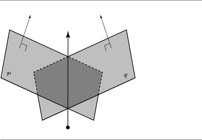
Figure 11.20 A ray represented as the intersection of two planes.

then (following Martin et al. 2000) we can deﬁne our planes as

: {P |P

[

P 1

]

= 0}

: {P |P

[

P 1

]

= 0}

where

[

n

]

[

n

]

See Figure 11.20.

There are an inﬁnite number of planes that include L(t), all of which have n

⊥

one convenient way to choose ˆn

is to set one of n

, n

,orn

to zero, and “perp”

(see Section 4.4.4) the other two; the best solution is generally agreed to be to set the

component of largest magnitude to zero:

n



[

−d

]

if |d

| > |d

| and |d

| > |d

[

0 d

−d

]

otherwise

11.4 Linear Components and Polynomial Surfaces 525

As it is computationally advantageous to have P

and P

orthogonal, we set

n

=n

We can complete our plane equations by noting that both P

and P

must contain

the ray origin P , and so we can set

=−n

· P

=−n

· P

Our (rational) B

ezier surface is deﬁned as

Q(u, v) =



i=0



j=0

(u)B

(v)w



i=0



j=0

(u)B

(v)w

where P

are the B

ezier control points and w

are the weights.

The intersection of a plane P

and the B

ezier patch can be represented by substi-

tution:

(u, v) =



i=0



j=0

(u)B

(v)w

[

n

]

)

[

n

]

[

Q(u, v) 1

]

= 0

for k ∈{0, 1}.

As any intersection point of the ray and the patch is on the ray, and the ray is

on both planes P

and P

, that intersection point must be on both planes; thus, the

intersection point must satisfy both

[

n

]

[

Q(u, v) 1

]

= 0

[

n

]

[

Q(u, v) 1

]

= 0

Kajiya (1982) recommends Laguerre’s method for solving this pair of implicit equa-

tions, while Martin et al. (2000) and Sweeney and Bartels (1986) use Newton

iteration.

Suppose we have an initial guess of (u

, v

); Newton’s method starts with these

values and iteratively reﬁnes them

→ u

→···→u

→ u

λ+1

→···

→ v

→···→v

→ v

λ+1

→···

by repeatedly solving the 2 ×2system

526 Chapter 11 Intersection in 3D



∂S

∂u

∂S

∂v

∂S

∂u

∂S

∂v





δu

λ+1

δv

λ+1





, v

)

, v

)



to produce

λ+1

= u

− δu

λ+1

= v

− δv

λ+1

Once one or more of several conditions are met, the Newton iteration concludes,

and the solution consists of the pair (u

λ+1

, v

λ+1

), or we conclude that the ray missed

the patch. Both Martin et al. (2000) and Sweeney and Bartels (1986) use a simple

“success” criterion—plug the (u

λ+1

, v

λ+1

) into S

and S

, and compare the sum to

some predetermined tolerance:

S

λ+1

, v

λ+1

)+S

λ+1

, v

λ+1

) <1

We conclude that the ray missed the surface if any one of several other conditions are

encountered:

i. The iteration takes us outside the bounds of the surface:

λ+1

min

or u

λ+1

max

λ+1

min

or v

λ+1

max

ii. The iteration degrades, rather than improves, the solution:

S

λ+1

, v

λ+1

)+S

λ+1

, v

λ+1

) > S

, v

)+S

, v

)

iii. The number of iterations has exceeded some preset limit.

Use of Bounding Volumes

Two observations motivate the use of bounding volumes: ﬁrst, Newton iteration

can converge quadratically to a root; second, bounding volumes have proven to

be generally useful in intersection tests because they allow for quick rejection and

thus can help avoid many expensive intersection computations. These seemingly

unrelated observations actually work together quite nicely if we can manage to make

the bounding volumes do a double duty of providing us with our initial guesses for

the Newton iteration.

The Chebyshev boxing described in Fournier and Buchanan (1984) was one ex-

ample of this, but, as Campagna, Slusallek, and Seidel (1997) point out, the Cheby-

shev polynomials only allow for integral patches. Both Martin et al. (2000) and

11.4 Linear Components and Polynomial Surfaces 527

Sweeney and Bartels (1986) use axis-aligned bounding boxes because they are sim-

ple to compute and efﬁcient to intersect with a ray. Both approaches begin by taking

a preprocessing step consisting of reﬁning the surface, using the Oslo algorithm (Co-

hen, Lyche, and Riesenfeld 1980; Goldman and Lyche 1993). In the case of Martin et

al. (2000), a heuristic is employed to estimate the number of additional knots to in-

sert; this heuristic takes into account estimates of the curvature and arc length. These

knots are then inserted, and each knot is increased in multiplicity up to the degree of

the patch in each of the directions; this results in a (rational) B

ezier patch between

each pair of distinct knots. The n × m control mesh for each B

ezier subpatch is then

bounded with an axis-aligned bounding box. These bounding boxes are then orga-

nized into a hierarchical structure.

In the case of Sweeney and Bartels (1986), the Oslo algorithm is again used

to reﬁne the surface. Their reﬁnement-level criteria are based on the (projected)

size of the quadrilateral facets induced by the reﬁnement, and whether the re-

ﬁned knots constitute “acceptably good starting guesses for the Newton iteration.”

They, too, build a hierarchy of bounding boxes, but their approach differs from

that of Martin et al. (2000): they start by creating a bounding box around each re-

ﬁned vertex, each of which overlaps its neighbors by some globally speciﬁed factor.

These overlapping bounding boxes are then combined into a hierarchy of bounding

volumes.

In either case, the leaf nodes of the hierarchy contain parameter values for the

regions of the surface they represent; in the method of Martin et al. (2000), the leaf

nodes contain the minimum and maximum parameter values (in each direction) for

the B

ezier (sub)patches they represent, and in the method of Sweeney and Bartels

(1986), the leaf nodes contain the parameter values associated with the reﬁned vertex.

In either case, the (u, v) parameter is used as the starting guess for the Newton

iteration, once it is determined that the ray has intersected a leaf’s bounding box.

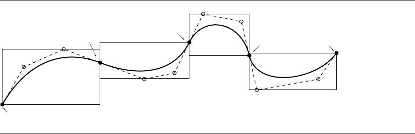
Figure 11.21 shows the basic idea of the use of bounding volumes for a curve,

for ease of illustration. The reﬁned vertices are shown in solid black; once these are

computed, the multiplicity of the knots is increased so that we get a B

ezier (sub)curve

between each pair of reﬁned vertices. The control points for each (sub)curve then are

used to deﬁne an axis-aligned bounding box, and the parameter values associated

with the control points serve as the initial guess for the Newton iteration, once a ray

has been determined to intersect a leaf ’s bounding box.

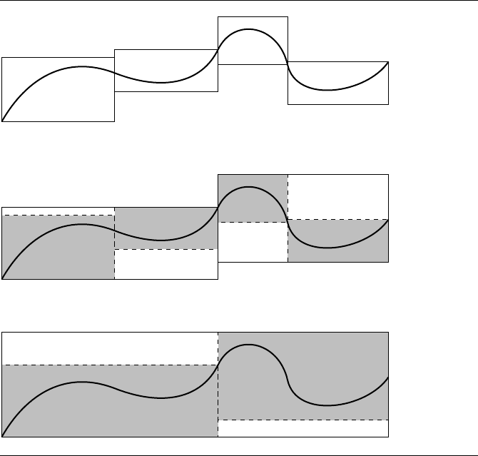
Figure 11.22 shows how the hierarchy of bounding boxes can be built up from the

leaf nodes—adjacent pairs of subcurve bounding boxes are combined into a higher-

level bounding box, and pairs of these are combined, and so on, until the hierarchy is

capped with a single bounding box that encompasses the entire surface.

An alternative to using the Oslo algorithm for the reﬁnement would be to use

an adaptive subdivision algorithm. The usual trade-offs apply—an adaptive subdivi-

sion scheme will generally produce a “better” tessellation of the surface, in that the

number of points of evaluation and their relative positioning will more accurately

reﬂect the scale and curvature of the surface, but at a cost of efﬁciency (the prepro-

cessing step will be slower). However, this cost may be more than made up for in the

528 Chapter 11 Intersection in 3D

u = 0.2

u = 0.6

u = 0.9

u = 1.1 u = 1.6

Figure 11.21 Leaf-node bounding boxes are constructed from the B

ezier polygon between each pair of

reﬁned vertices.

actual intersection tests, as the bounding box hierarchy will tend to better reﬂect the

geometry of the surface.

An outline for this algorithm is as follows:

1. Preprocess the surface:

a. Reﬁne or adaptively subdivide the surface until some ﬂatness criteria are met.

At each control point interpolating the surface, save the parameter values for

that point.

b. For each span of the reﬁned surface, create an axis-aligned bounding box

using the control points of the region. Associate with each box the parameters

(in each direction) that the region represents.

c. Recursively coalesce neighboring bounding boxes into a hierarchy.

2. Intersect:

a. Intersect the ray with the bounding box hierarchy.

b. When the ray intersects a leaf node, set initial guess for (u

, v

) using the

parametric ranges stored with the bounding box. A good choice might be to

use the midpoint of the range: u

= (u

min

+ u

max

)/2, and similarly for v

c. Repeatedy apply the Newton iteration step until convergence criterion is met

or ray is determined to have missed the surface.

Martin et al. (2000) describe how this basic approach can be extended to handle

trim curves: the orientation of each trim curve is analyzed to determine if it deﬁnes

a hole or an island; then, each trim curve is placed in a node, and since trim curves

can be nested, a hierarchy of nodes is created. Once a ray intersection is detected, the

intersection is checked against the trimming hierarchy to see if it is to be culled or

returned as a hit.

11.5 Planar Components 529

Figure 11.22 Adjacent bounding boxes are coalesced into a single box at the next level in the

hierarchy.

11.5 Planar Components

In this section, we discuss the problem of computing intersections of planar

components—triangles and planes.

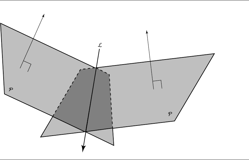
11.5.1 Two Planes

The intersection of two planes, if it exists (parallel planes don’t intersect, but all others

do), is a line L (see Figure 11.23). If we have two planes

530 Chapter 11 Intersection in 3D

Figure 11.23 Intersection of two planes.

: n

· P =s

: n

· P =s

then that line has direction

n

×n

To completely specify the intersection line, we need a point on that line. Suppose

the point is a linear combination of n

and n

, with these normal vectors considered

as points:

P = a n

+ bn

That point has to be on both planes, and so must satisfy both plane equations

n

· P =s

n

· P =s

11.5 Planar Components 531

yielding

an



+ bn

·n

= s

a n

·n

+ bn



= s

Solving for a and b,wehave

a =

n

·n

− s

n



(n

·n

)

−n



n



b =

n

·n

− s

n



(n

·n

)

−n



n



giving us the line equation

L = P + t(n

×n

)

= (a n

+ bn

) + t(n

×n

)

Note that choosing the direction of the line to be n

×n

instead will give you the

same line, but with reversed direction.

The pseudocode is

bool IntersectionOf2Planes(Plane3D p1, Plane3D p2, Line3D line)

{

Vector3D d = Cross(p1.normal,p2.normal)

if (d.length() == 0) {

return false;

}

line.direction = d;

float s1, s2, a, b;

s1 = p1.d; // d from the plane equation

s2 = p2.d;

float n1n2dot = Dot(p1.normal, p2.normal);

float n1normsqr = Dot(p1.normal, p1.normal);

float n2normsqr = Dot(p2.normal, p2.normal);

a = (s2 * n1n2dot - s1 * n2normsqr) / (n1n2dot^2 - n1normsqr * n2normsqr);

b = (s1 * n1n2dot - s2 * n2normsqr) / (n1n2dot^2 - n1normsqr * n2normsqr);

line.p=a*p1.normal+b*p2.normal;

return true;

}

532 Chapter 11 Intersection in 3D

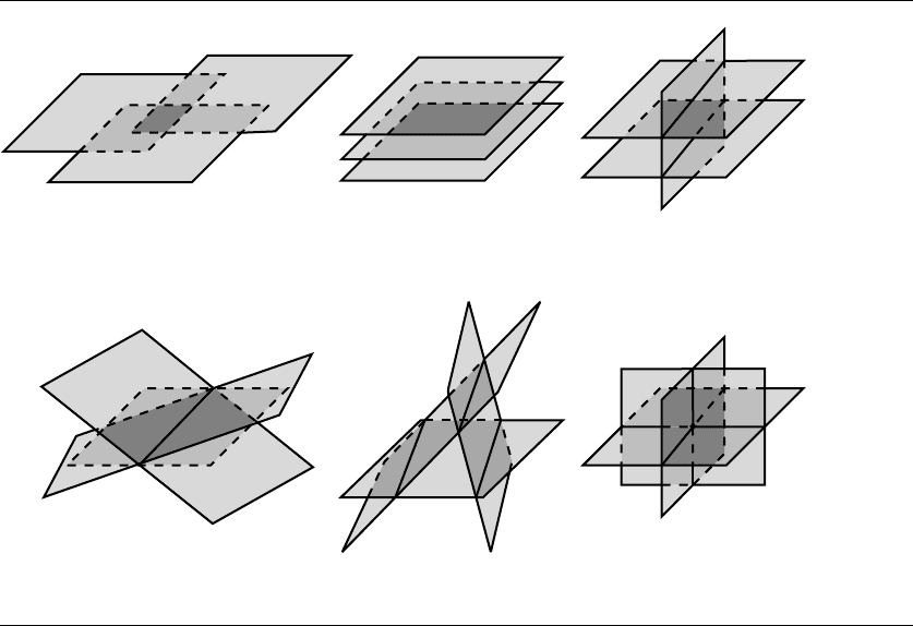
(a) (b) (c)

(d) (e) (f)

Figure 11.24 Possible conﬁgurations for three planes described in Table 11.1.

11.5.2 Three Planes

The problem of intersecting three planes is quite similar to that of intersecting two

planes, but there are more cases to consider, and it is useful to distinguish between

them. Given three planes

: {P

, n

}

: {P

, n

}

: {P

, n

}

there are six possible conﬁgurations, as shown in Figure 11.24. Following Dan Sun-

day’s taxonomy (Sunday 2001c), we can describe each conﬁguration in terms of inter-

section (or not) and the vector algebraic condition characterizing it (see Table 11.1).

A bit of explanation may be in order: if any planes P

and P

are parallel, then

their normals are the same, which can be expressed as

11.5 Planar Components 533

Table 11.1

The six possible conﬁgurations of three planes can be distinguished by testing

vector algebraic conditions.

Conﬁguration Intersection? Condition

All planes parallel n

×n

= 0, ∀i, j ∈{0, 1, 2}

Coincident (Figure 11.24a) Plane n

· P

=n

· P

=n

· P

Disjoint (Figure 11.24b) None n

· P

=n

· P

=n

· P

Only two planes parallel

(Figure 11.24c) Two parallel lines Only one n

×n

= 0, ∀i, j ∈{0, 1, 2}

(or coincident) (or one line)

No two planes parallel n

×n

= 0, ∀i, j ∈{0, 1, 2}, i = j

Intersection lines parallel n

· (n

×n

) = 0

Coincident (Figure 11.24d) One line Test point from one line

Disjoint (Figure 11.24e) Three parallel lines

Intersection lines nonparallel

(Figure 11.24f) Point n

· (n

×n

) = 0

n

×n

= 0

Further, if P

and P

are coincident, then any point on P

will also be on P

, which

can be expressed as

n

· P

=n

· P

These conditions allow us to distinguish between the ﬁrst three cases and to distin-

guish between them and the other cases.

If no two planes are parallel, then one of conﬁgurations (d), (e), or (f) holds. In

order to distinguish (f) from the other two, we note that P

and P

must meet in a

line, and that line must intersect P

in a single point. As we saw in the problem of the

intersection of two planes, the line of intersection has a direction vector equal to the

cross product of the normals of those two planes; that is, n

×n

.IfP

is to intersect

that line in a single point, then its normal n

cannot be orthogonal to that line. Thus,

the three planes intersect if and only if

n

· (n

×n

) = 0

This last equation should be recognized as the scalar triple product (see Section 3.3.2),

which is the determinant of the 3 × 3 matrix of coefﬁcients of the planes’ normals.

Goldman (1990a) condenses the computation of the point of intersection to

P = ((P

·n

)(n

×n

) + (P

·n

)(n

×n

) + (P

·n

)(n

×n

))/n

· (n

×n

)