Schneider P., Eberly D.H. Geometric Tools for Computer Graphics
Подождите немного. Документ загружается.

674 Chapter 13 Computational Geometry Topics
P
1
P
3
C
1
C
2
C
3
C
4
P
2
C
0
P
0
+
+
–
–
+
+
–
–
P
1
P
3
C
1
C
2
C
3
C
4
P
2
C
0
P
0
+–
+–
+–
+–
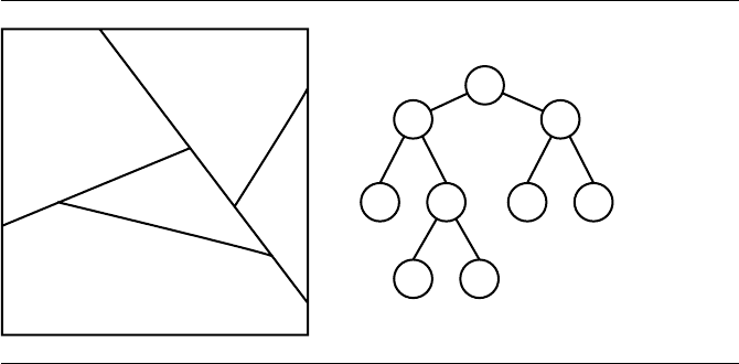
Figure 13.1 BSP tree partitioning of the plane.
side.” If X is on the negative side, then n · X −c<0.ApointX on the line of course
satisfies n · X −c =0.
Each half-plane may be further subdivided by another line in the plane. The
resulting positive and negative regions can themselves be subdivided. The resulting
partitioning of the plane is represented by a binary tree, each node representing the
splitting line. The left child of a node corresponds to the positive side of the splitting
line that the node represents; the right child corresponds to the negative side. The
leaf nodes of the tree represent the convex regions obtained by the partitioning.
Figure 13.1 illustrates this. The square is intended to represent all of the plane. The
partitioning lines are labeled with P , and the convex regions are labeled with C.
13.1.1 BSP Tree Representation of a Polygon
A BSP tree represents a partitioning of the plane, but it can also be used to partition
polygons into convex subpolygons. The decomposition can be used in various ways.
The tree supports point-in-polygon queries, discussed later in this section. Other
algorithms for point-in-polygon queries are discussed in Section 13.3. A BSP tree
represents a general decomposition of a polygon into triangles—the idea explored
in Section 13.9. Finally, BSP tree representations for polygons can be used to support
Boolean operations on polygons—the idea explored in Section 13.5.
The simplest way to construct a BSP tree for a polygon is to create the nodes
so that each represents a splitting line that contains an edge of the polygon. Other
polygon edges are split at a node by using the splitting line. Any subedges that are on
the positive side of a line are sent to the positive child, and the process is repeated.
Any subedges that are on the negative side are sent to the negative child, and the
13.1 Binary Space-Partitioning Trees in 2D 675
process is repeated. It is possible that another polygon edge is fully on the splitting
line. Such edges, called coincident edges, are also stored at the node representing the
splitting line. In this construction, at least one edge of the polygon is contained by
the splitting line. It is not necessary to require that the splitting lines contain polygon
edges. We will revisit this idea later in the section. The pseudocode for construction
of a BSP tree from a polygon is listed below. The input list for the top-level call is the
collection of edges from the polygon, assumed to be nonempty.
BspTree ConstructTree(EdgeList L)
{
T = new BspTree;
// use an edge to determine the splitting line for the tree node
T.line = GetLineFromEdge(L.first); // Dot(N, X)-c=0
EdgeList posList, negList; // initially empty lists
for (each edge E of L) {
// Determine how edge and line relate to each other. If the edge
// crosses the line, the subedges on the positive and negative
// side of the line are returned.
type = Classify(T.line, E, SubPos, SubNeg);
if (type is CROSSES) {
// Dot(N, X)-c<0foronevertex, Dot(N, X)-c>0
// for the other vertex
posList.AddEdge(SubPos);
negList.AddEdge(SubNeg);
} else if (type is POSITIVE) {
// Dot(N, X)-c>=0forboth vertices, at least one positive
posList.AddEdge(E);
} else if (type is NEGATIVE) {
// Dot(N, X)-c<=0forboth vertices, at least one negative
negList.AddEdge(E);
} else {
// type is COINCIDENT
// Dot(N, X)-c=0forboth vertices
T.coincident.AddEdge(E);
}
}
if (posList is not empty)
T.posChild = ConstructTree(posList);
else
T.posChild = null;
676 Chapter 13 Computational Geometry Topics
e
1
e
0
n
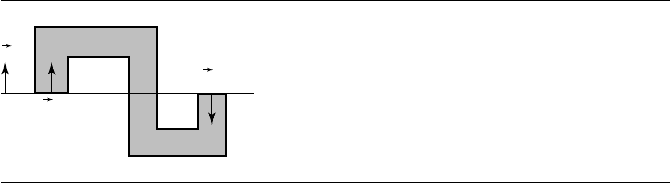
Figure 13.2 A partitioning line for which two coincident edges have opposite direction normals.
if (negList is not empty)
T.negChild = ConstructTree(negList);
else
T.negChild = null;
return T;
}
The function GetLineFromEdge produces a line whose normal vector points to the
outside region of the polygon at the specified edge. Other coincident edges may or
may not have normals that point in the same direction as the line normal. Figure
13.2 shows such a situation.
The function
Classify tries to find a point of intersection of the current edge and
the node’s line. If there is an intersection that is an interior point of the edge, the
positive and negative subedges are returned. It is possible that one end point of the
edge is on the line, but the other end point is not. In this case, the edge is classified as
either a positive edge or a negative edge. Of course the edge can be fully on one side
or the other without intersecting the line at all, in which case the edge is classified as
either positive or negative. Finally, the edge can be entirely on the splitting line, in
which case the edge is classified as coincident. The pseudocode for this function is
int Classify(Line L, Edge E, Edge SubPos, Edge SubNeg)
{
d0 = Dot(L.normal, E.V(0) - L.origin);
d1 = Dot(L.normal, E.V(1) - L.origin);
if(d0*d1<0){
// edge crosses line
t = d0 / (d0 - d1);
I = E.V(0)+t*(E.V(1) - E.V(0));
if(d1>0){
SubNeg = Edge(E.V(0), I);
SubPos = Edge(I, E.V(1));
13.1 Binary Space-Partitioning Trees in 2D 677
} else {
SubPos = Edge(E.V(0), I);
SubNeg = Edge(I, E.V(1));
}
return CROSSES;
} else if (d0>0ord1>0){
// edge on positive side of line
return POSITIVE;
} else if (d0<0ord1<0){
// edge on negative side of line
return NEGATIVE;
} else {
// edge is contained by the line
return COINCIDENT;
}
}
Because of floating-point round-off errors, it is possible that d
0
d
1
< 0, but t is
nearly zero (or one) and may as well be treated as zero (or one). An implementation
of
Classify should include such handling to avoid the situation where two edges meet
at a vertex; the first edge is used for the splitting line, and numerically the second edge
appears to be crossing the line, thereby causing a split when there should be none.
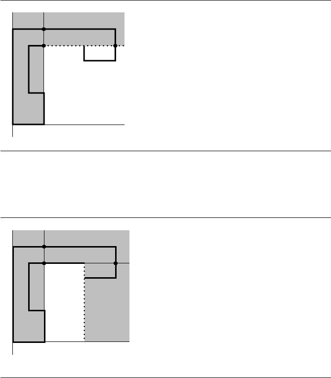
Example Figure 13.3 shows an inverted L-shaped polygon that has 10 vertices and 10 edges.
Theverticesareindexedfrom0to9.Theedgesare9, 0 and i, i + 1 for 0 ≤ i ≤ 8.
We construct the BSP tree an edge at a time. At each step the splitting line is shown
as dotted, the positive side region is shown in white, and the negative side region is
shown in gray.
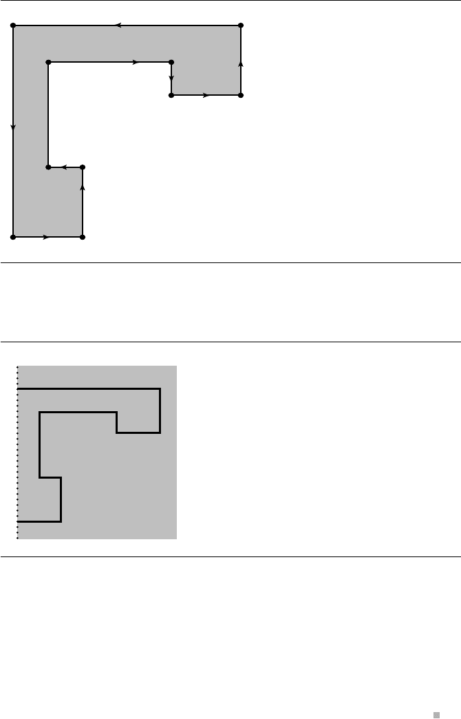
The first edge to be processed is 9, 0. Figure 13.4 shows the partitioning of the
plane by a dotted line containing the edge and the root node (r)ofthetree.Theedge
9, 0is part of that node (the edge defines the splitting line) and the positive (p) and
negative (n) edges created by the splitting. In this case, all remaining edges are on the
negative side of the line.
The next edge to be processed is 0, 1. Figure 13.5 shows the state of the BSP tree
after the edge is processed.
The next edge to be processed is 1, 2. Figure 13.6 shows the state of the BSP tree
after the edge is processed. The edge forces a split of both 4, 5 and 8, 9, causing
the introduction of new vertices labeled as 10 and 11 in the figure.
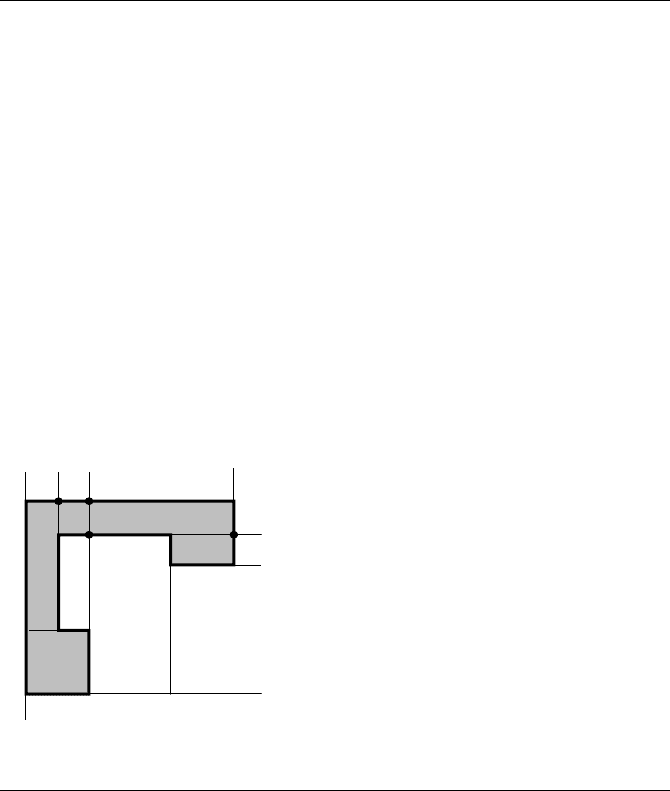
The next edge to be processed is 10, 5. Figure 13.7 shows the state of the BSP tree
after the edge is processed. The edge forces a split of 7, 8, causing the introduction
of the new vertex labeled as 12 in the figure.
The next edge to be processed is 5, 6. Figure 13.8 shows the state of the BSP tree
after the edge is processed. No new vertices are introduced by this step.
678 Chapter 13 Computational Geometry Topics
2
3
45
67
10
98
Figure 13.3 A sample polygon for construction of a BSP tree.
2
3
4
5
67
10
9
8
+ –
R
0
r <9,0>
p [region 0]
n <0,1>,<1,2>,<2,3>,<3,4>,<4,5>,
<5,6>,<6,7>,<7,8>,<8,9>
Figure 13.4
Current state after processing edge 9, 0.
We leave it to you to verify that the remaining edges to be processed are 6, 7,
7, 12, 12, 8, 8, 11, 2, 3, 3, 4 (forcing a split of 11, 9 and introducing a new
vertex labeled as 13), 4, 10, 11, 13, and 13, 9. The final state of the BSP tree is
shown in Figure 13.9. The regions corresponding to the leaf nodes of the BSP tree
are labeled in the figure. The new vertices in the partitioning are shown as black dots.
The point 13 introduced in the split of 11, 9is the leftmost one in the figure.
13.1 Binary Space-Partitioning Trees in 2D 679
2
3
45
67
01+
–
9
8
+ –
R
0
R
1
r <9,0>
p [region 0]
n <0,1>
p [region 1]
n <1,2>,<2,3>,<3,4>,<4,5>,
<5,6>,<6,7>,<7,8>,<8,9>
Figure 13.5 Current state after processing edge 0, 1.
2
3
410
11
5
67
01+
– +
–
9
8
+ –
R
0
R
1
r <9,0>
p [region 0]
n <0,1>
p [region 1]
n <1,2> {split<4,5>:<4,10>,<10,5>,
<8,9>:<8,11><11,9>}
p <10,5>,<5,6>,<6,7>,<7,8>,<8,11>
n <2,3>,<3,4>,<4,10>,<11,9>
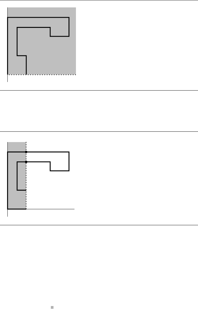
Figure 13.6 Current state after processing edge 1, 2. This edge forces a split of 4, 5 to 4, 10
and 10, 5. It also forces a split of 8, 9 to 8, 11 and 11, 9.
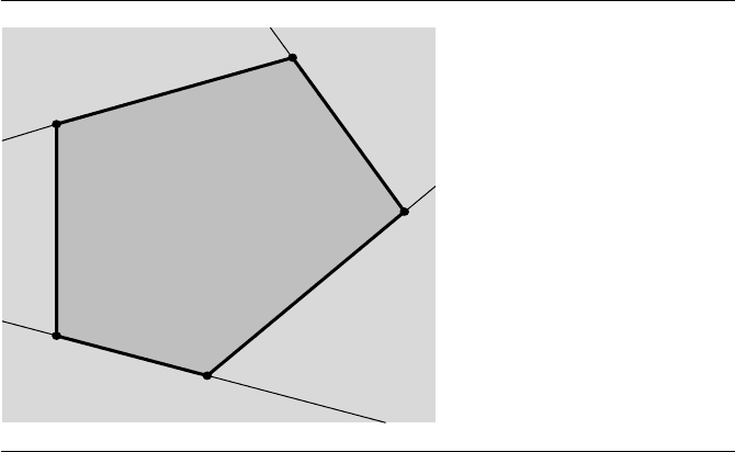
Example
Figure 13.10 shows a partitioning of space for a convex polygon and the correspond-
ing BSP tree. The tree construction for the convex polygon requires no splitting of
edges. However, the tree is just a linear list of nodes. Any tests for containment inside
the polygon, in the worst case, require processing at every node of the tree. A better
situation for minimizing the processing is to start with a binary tree that is balanced
as much as possible.
680 Chapter 13 Computational Geometry Topics
2
3
410 12
11
5
67
01+
– +
–
+
–
9
8
+ –
R
0
R
1
r <9,0>
p [region 0]
n <0,1>
p [region 1]
n <1,2>
p <10,5> {split<7,8>:<7,12><12,8>}
p <5,6>,<6,7>,<7,12>
n <12,8>,<8,11>
n <2,3>,<3,4>,<4,10>,<11,9>
Figure 13.7 Current state after processing edge 10, 5. This edge forces a split of 7, 8 to 7, 12
and 12, 8.
2
3
410 12
11
5
6
7
01+
– +
–
+
–
9
8
+ –
+ –
R
0
R
2
R
1
r <9,0>
p [region 0]
n <0,1>
p [region 1]
n <1,2>
p <10,5>
p <5,6>
p [region 2]
n <6,7>,<7,12>
n <12,8>,<8,11>
n <2,3>,<3,4>,<4,10>,<11,9>
Figure 13.8 Current state after processing edge 5, 6.
13.1.2 Minimum Splits versus Balanced Trees
As we saw in the example of a BSP tree for a convex polygon, the tree construction
required no splitting, but the tree is very unbalanced since it is a linear list. The
problem in the construction is that the splitting lines were selected to contain edges
of the polygon. That constraint is not necessary for partitioning space by a polygon.
An alternative is to choose splitting lines in a clever way to obtain minimum splitting
and a balanced tree. For a convex polygon, it is always possible to build such a tree.
13.1 Binary Space-Partitioning Trees in 2D 681
– +
– +
– +
– +
–
+
–
+
–
+
–
+
+
–
+
–
+
–
+ –
+ –
R
0
R
9
R
10
R
14
R
12
R
11
R
5
R
2
R
3
R
8
R
4
R
6
R
7
R
13
R
1
r <9,0>
p [region 0]
n <0,1>
p [region 1]
n <1,2>
p <10,5>
p <5,6>
p [region 2]
n <6,7>
p [region 3]
n <7,12>
p [region 4]
n [region 5]
n <12,8>
p [region 6]
n <8,11>
p [region 7]
n [region 8]
n <2,3>
p <3,4>
p <4,10>
p [region 10]
n <11,13>
p [region 11]
n [region 12]
n <13,9>
p [region 13]
n [region 14]
n [region 9]
+
–
Figure 13.9
Final state after processing edge 13, 9.
For general polygons, it is not clear what the best strategy is for choosing the splitting
lines.
For a convex polygon, a bisection method works very well. The idea is to choose
a line that contains vertex V
0
and another vertex V
m
that splits the vertices into two
subsets of about the same number of elements. A routine to compute m was given in
Section 7.7.2 for finding extreme points of convex polygons:
682 Chapter 13 Computational Geometry Topics
R
4
R
0
R
1
R
5
R
2
R
3
4
0
1
2
3
r <0,1>
p [region 0]
n <1,2>
p [region 1]
n <2,3>
p [region 2]
n <3,4>
p [region 3]
n <4,0>
p [region 4]
n [region 5]
Figure 13.10 Partition for a convex polygon and the corresponding BSP tree.
int GetMiddleIndex(int i0, int i1, int N)
{
if (i0 < i1)
return (i0 + i1) / 2;
else
return (i0 + i1 + N) / 2 (mod N);
}
The value N is the number of vertices. The initial call sets both i
0
and i
1
to zero.
The condition when i
0
<i
1
has an obvious result—the returned index is the average
of the input indices, certainly supporting the name of the function. For example, if
the polygon has N = 5 vertices, inputs i
0
= 0 and i
1
= 2 lead to a returned index of
1. The other condition handles wraparound of the indices. If i
0
= 2 and i
1
= 0, the
implied set of ordered indices is {2, 3, 4, 0}. The middle index is selected as 3 since
3 = (2 +0 +5)/2 (mod 5).
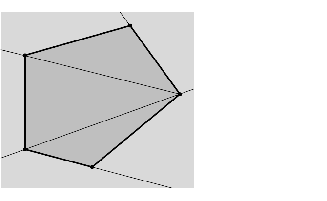
Because the splitting line passes through vertices and because the polygon is con-
vex, no edges are split by this line. Because of the bisection, the tree will automatically
be balanced. Figure 13.11 shows the partitioning and BSP tree for the convex poly-
gon of the last example. Observe that the depth of this tree is smaller than that of the
original construction.
13.1 Binary Space-Partitioning Trees in 2D 683
R
6
R
0
R
1
R
2
R
7
R
5
R
3
R
4
4
0
1
2
3
r <0,2>
p <0,1>
p [region 0]
n <1,2>
p [region 1]
n [region 2]
n <2,4>
p <2,3>
p [region 3]
n <3,4>
p [region 4]
n [region 5]
n <4,0>
p [region 6]
n [region 7]
+
–
+
–
–
+
–
+
+ –
– +
Figure 13.11 Partition for a convex polygon and the corresponding balanced BSP tree.
13.1.3 Point in Polygon Using BSP Trees
A BSP tree representation of a polygon naturally provides the ability to test if a point
is inside, outside, or on the polygon. The point is processed at each node of the tree
by testing which side of the splitting line it is on. If the processing reaches a leaf node,
the point is in the corresponding convex region. If that region is inside (or outside)
the polygon, then the point is inside (or outside) the polygon. At any node if the
point is on an edge contained by the splitting line, then the point is, of course, on the
polygon itself. The pseudocode is listed below. The return value of the function is +1
if the point is outside, −1 if the point is inside, or 0 if the point is on the polygon.
int PointLocation(BspTree T, Point P)
{
// test point against splitting line
type = Classify(T.line, P);
if (type is POSITIVE) {
if (T.posChild exists)
return PointLocation(T.posChild, P);
else
return +1;
} else if (type is NEGATIVE) {
if (T.negChild exists)
return PointLocation(T.negChild, P);