Smith R., Minton R. Calculus
Подождите немного. Документ загружается.

P1: OSO/OVY P2: OSO/OVY QC: OSO/OVY T1: OSO
MHDQ256-Ch09 MHDQ256-Smith-v1.cls December 17, 2010 19:47
LT (Late Transcendental)
CONFIRMING PAGES
9-83 SECTION 9.9
..
Fourier Series 613
and the series
∞
k=1
4
π(2k − 1)
2
converges. (Hint: Compare this last series to the
convergent p-series
∞
k=1
1
k
2
, using the Limit Comparison Test.) To get an idea of the
function to which the series converges, we plot several of the partial sums of the
series,
F
n
(x) =
π
2
−
n
k=1
4
π(2k − 1)
2
cos[(2k − 1)x].
y
3
2
p 2pp2p3p4p 3p 4p
x
y
3
2
p 2pp2p3p4p 3p 4p
x
FIGURE 9.48a
y = F
1
(x) and y = f (x)
FIGURE 9.48b
y = F
2
(x) and y = f (x)
y
3
2
p 2pp2p3p4p 3p 4p
x
y
3
2
p 2pp2p3p4p 3p 4p
x
FIGURE 9.48c
y = F
4
(x) and y = f (x)
FIGURE 9.48d
y = F
8
(x) and y = f (x)
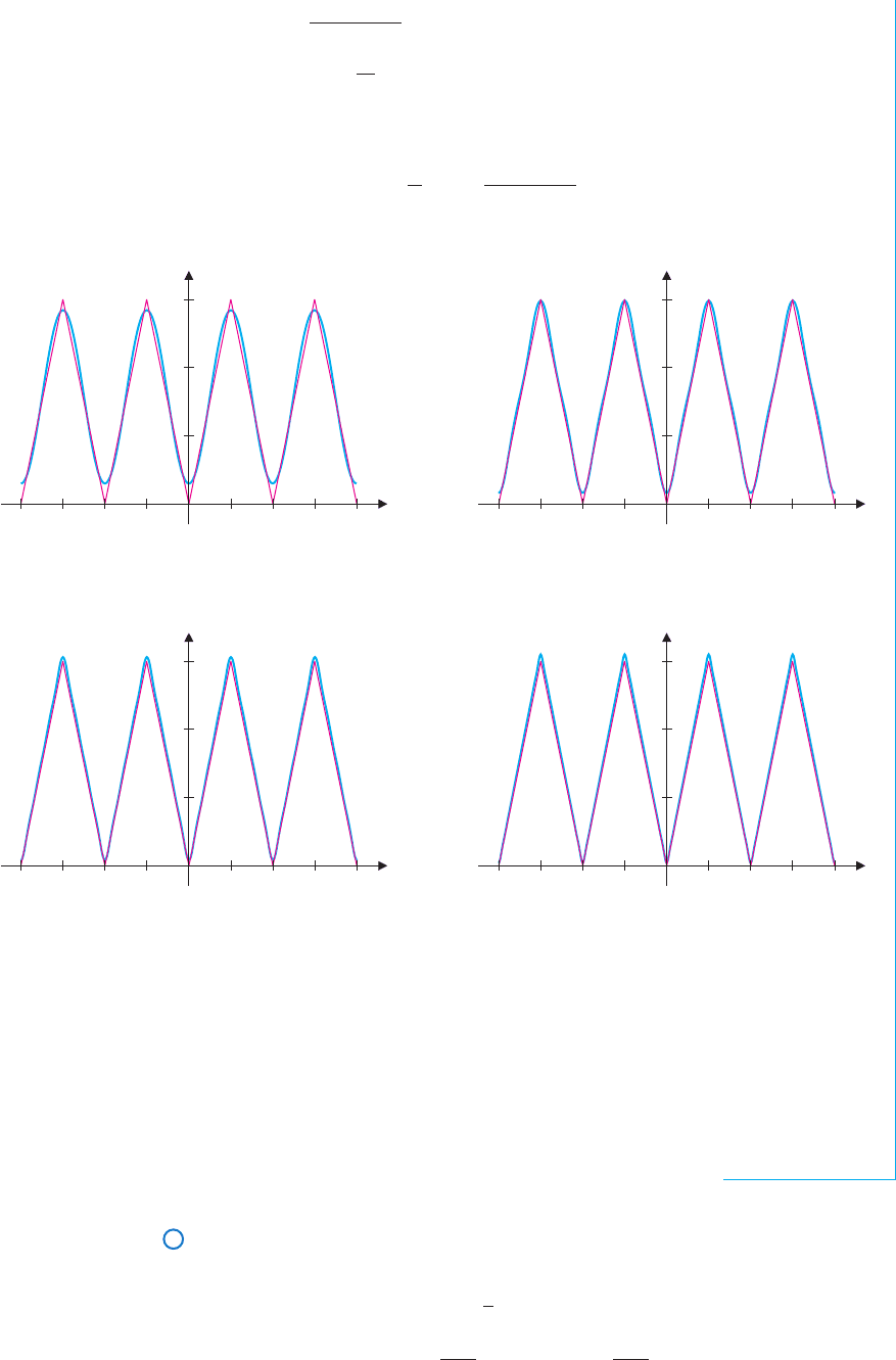
See if you can conjecture the sum of the series by looking at Figures 9.48a–d. Notice
how quickly the partial sums of the series appear to converge to the triangular-wave
function f (shown in red; also see Figure 9.47). We’ll see later that the Fourier series
converges to f (x) for all x. There’s something further to note here: the accuracy of the
approximation is fairly uniform. That is, the difference between a given partial sum and
f (x) is roughly the same for each x. Take care to distinguish this behavior from that of
Taylor polynomial approximations, where the farther you get away from the point about
which you’ve expanded, the worse the approximation tends to get.
Functions of Period Other Than 2π
Fora function f that is periodic of period T = 2π,we want to expand f in a series of simple
functions of period T. First, define l =
T
2
and notice that
cos
kπ x
l
and sin
kπ x
l
P1: OSO/OVY P2: OSO/OVY QC: OSO/OVY T1: OSO
MHDQ256-Ch09 MHDQ256-Smith-v1.cls December 17, 2010 19:47
LT (Late Transcendental)
CONFIRMING PAGES
614 CHAPTER 9
..
Infinite Series 9-84
are periodic of period T = 2l, for each k = 1, 2,....The Fourier series expansion of f of
period 2l is then
a
0
2
+
∞
k=1
a
k
cos
kπ x
l
+ b
k
sin
kπ x
l
.
We leave it as an exercise to show that the Fourier coefficients in this case are given by the
Euler-Fourier formulas:
a
k
=
1
l
l
−l
f (x) cos
kπ x
l
dx, for k = 0, 1, 2,... (9.7)
and
b
k
=
1
l
l
−l
f (x) sin
kπ x
l
dx, for k = 1, 2, 3,.... (9.8)
Notice that (9.3), (9.5) and (9.6) are equivalent to (9.7) and (9.8) with l = π.
EXAMPLE 9.3 A Fourier Series Expansion for a Square-Wave Function
Find a Fourier series expansion for the function
f (x) =
−2, if −1 < x ≤ 0
2, if 0 < x ≤ 1
,
where f is defined so that it is periodic of period 2 outside of the interval [−1, 1].
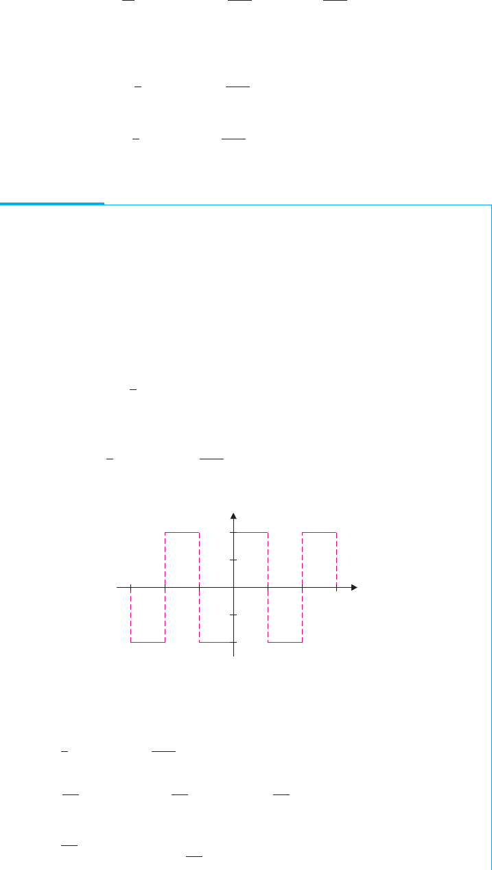
Solution The graph of f is the square wave seen in Figure 9.49. From the
Euler-Fourier formulas (9.7) and (9.8) with l = 1, we have
a
0
=
1
1
1
−1
f (x) dx =
0
−1
(−2) dx +
1
0
2dx = 0.
Likewise, we get
a
k
=
1
1
1
−1
f (x) cos
kπ x
1
dx = 0, for k = 1, 2, 3,....
y
x
1 2 3123
2
1
1
2
FIGURE 9.49
Square wave
Finally, we have
b
k
=
1
1
1
−1
f (x) sin
kπ x
1
dx =
0
−1
(−2)sin(kπ x)dx +
1
0
2sin(kπ x)dx
=
2
kπ
cos(kπ x)
0
−1
−
2
kπ
cos(kπ x)
1
0
=
4
kπ
[cos0 −cos(kπ)]
=
4
kπ
[1 − cos(kπ )] =
⎧
⎨
⎩
0, if k is even
8
kπ
, if k is odd
.
Since cos(kπ) = 1 when k is even,
and cos(kπ) =−1 when k is odd.
P1: OSO/OVY P2: OSO/OVY QC: OSO/OVY T1: OSO
MHDQ256-Ch09 MHDQ256-Smith-v1.cls December 17, 2010 19:47
LT (Late Transcendental)
CONFIRMING PAGES
9-85 SECTION 9.9
..
Fourier Series 615
This gives us the Fourier series
a
0
2
+
∞
k=1
[a
k
cos(kπ x) + b
k
sin(kπ x)] =
∞
k=1
b
k
sin(kπ x) =
∞
k=1
b
2k−1
sin[(2k − 1)π x]
=
∞
k=1
8
(2k − 1)π
sin[(2k − 1)π x].
Since b
2k
= 0 and b
2k−1
=
8
(2k − 1)π
.
Although we as yet have no tools for determining the convergence or divergence of this
series, we graph a few of the partial sums of the series,
F
n
(x) =
n
k=1
8
(2k − 1)π
sin[(2k − 1)π x]
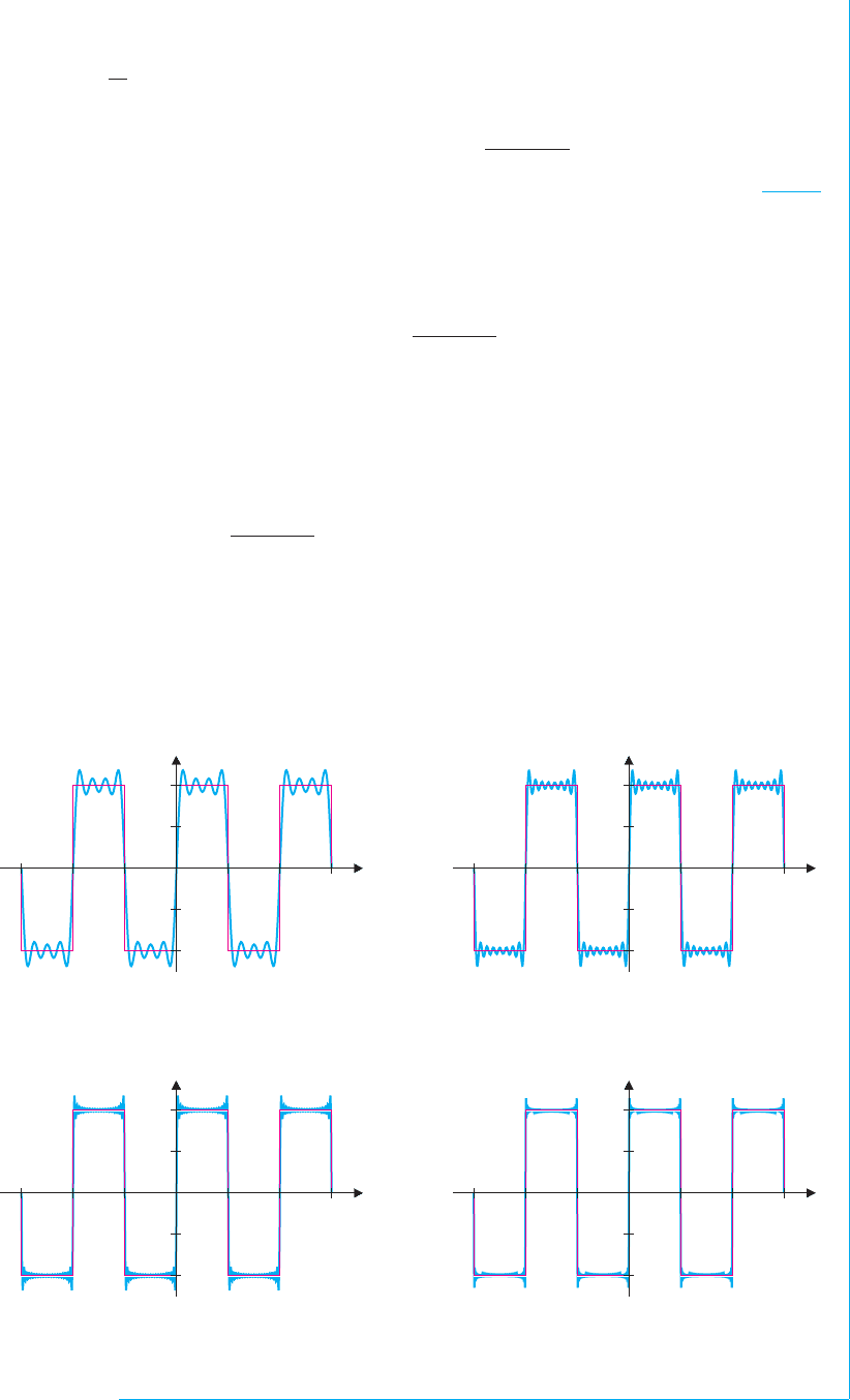
in Figures 9.50a–d. From the graphs, it appears that the series is converging to the
square-wave function f, except at the points of discontinuity, x = 0, ±1, ±2, ±3,....
At those points, the series appears to converge to 0. You can easily verify this by
observing that the terms of the series are
8
(2k − 1)π
sin[(2k − 1)π x] = 0, for integer values of x.
Since each term in the series is zero, the series converges to 0 at all integer values
of x. You might think of this as follows: at the points where f is discontinuous, the
series converges to the average of the two function values on either side of the
discontinuity. As we will see, this is typical of the convergence of Fourier series.
y
x
1 2 3123
2
1
1
2
y
x
1 2 3123
2
1
1
2
FIGURE 9.50a
y = F
4
(x) and y = f (x)
FIGURE 9.50b
y = F
8
(x) and y = f (x)
y
x
1 23123
2
1
1
2
y
x
1 2 3123
2
1
1
2
FIGURE 9.50c
y = F
20
(x) and y = f (x)
FIGURE 9.50d
y = F
50
(x) and y = f (x)

P1: OSO/OVY P2: OSO/OVY QC: OSO/OVY T1: OSO
MHDQ256-Ch09 MHDQ256-Smith-v1.cls December 17, 2010 19:47
LT (Late Transcendental)
CONFIRMING PAGES
616 CHAPTER 9
..
Infinite Series 9-86
We now state the following major result on the convergence of Fourier series.
THEOREM 9.1 (Fourier Convergence Theorem)
Suppose that f is periodic of period 2l and that f and f
are continuous on the interval
[−l, l], except for at most a finite number of jump discontinuities. Then, f has a
convergent Fourier series expansion. Further, the series converges to f (x), when f is
continuous at x and to
1
2
lim
t→x
+
f (t) + lim
t→x
−
f (t)
at any points x where f is discontinuous.
REMARK 9.1
The Fourier Convergence
Theorem says that a Fourier
series may converge to a
discontinuous function, even
though every term in the
series is continuous (and
differentiable) for all x.
The proof of the theorem is beyond the level of this text and can be found in texts on
advanced calculus or Fourier analysis.
EXAMPLE 9.4 Proving Convergence of a Fourier Series
Use the Fourier Convergence Theorem to prove that the Fourier series expansion of
period 2π,
π
2
−
∞
k=1
4
(2k − 1)
2
π
cos[(2k − 1)x],
derived in example 9.2, for f (x) =|x|, for −π ≤ x ≤ π and periodic outside of
[−π, π], converges to f (x) everywhere.
Solution First, note that f is continuous everywhere. (See Figure 9.47.) We also have
that since
f (x) =|x|=
−x, if −π ≤ x < 0
x, if 0 ≤ x <π
and is periodic outside [−π, π], then
f
(x) =
−1, −π<x < 0
1, 0 < x <π
.
So, f
is also continuous on [−π, π], except for jump discontinuities at x = 0 and
x =±π . From the Fourier Convergence Theorem, we now have that the Fourier series
converges to f (x) everywhere (since f is continuous everywhere). Because of this, we
write
f (x) =
π
2
−
∞
k=1
4
(2k − 1)
2
π
cos(2k − 1)x,
for all x.
As you can see from the Fourier Convergence Theorem, Fourier series do not always
converge to the function you are expanding.
EXAMPLE 9.5 Investigating Convergence of a Fourier Series
Usethe FourierConvergence Theorem toinvestigatethe convergenceoftheFourierseries
∞
k=1
8
(2k − 1)π
sin[(2k − 1)π x],
derived as an expansion of the square-wave function
f (x) =
−2, if −1 < x ≤ 0
2, if 0 < x ≤ 1
,
where f is taken to be periodic outside of [−1, 1]. (See example 9.3.)
P1: OSO/OVY P2: OSO/OVY QC: OSO/OVY T1: OSO
MHDQ256-Ch09 MHDQ256-Smith-v1.cls December 17, 2010 19:47
LT (Late Transcendental)
CONFIRMING PAGES
9-87 SECTION 9.9
..
Fourier Series 617
Solution First, note that f is continuous, except for jump discontinuities at
x = 0, ±1, ±2,....Further,
f
(x) =
0, if −1 < x < 0
0, if 0 < x < 1
and is periodic outside of [−1, 1]. Thus, f
is also continuous everywhere, except at
integer values of x where f
is undefined. From the Fourier Convergence Theorem,
the Fourier series will converge to f (x) everywhere, except at the discontinuities,
x = 0, ±1, ±2,...,where the series converges to the average of the one-sided limits,
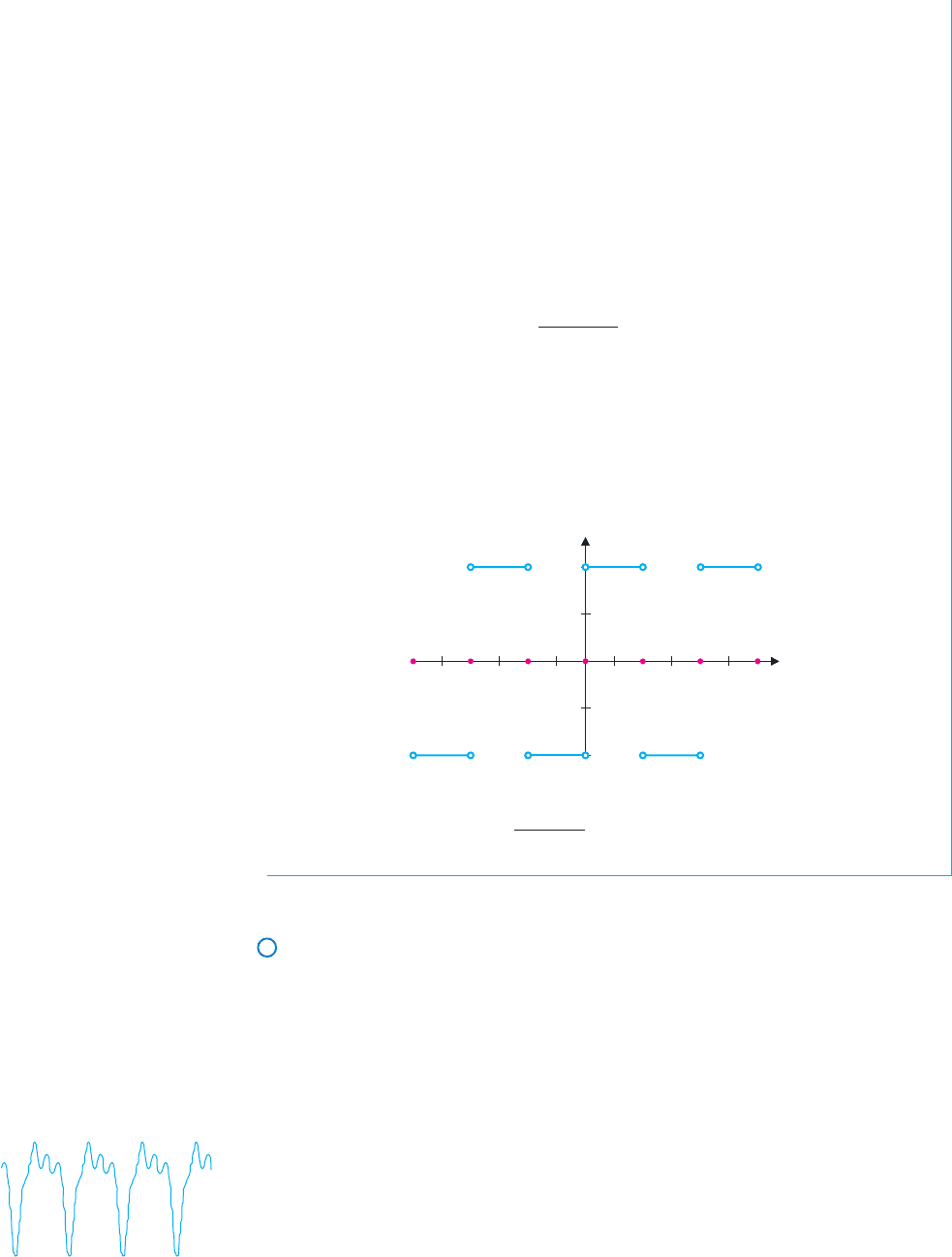
that is, 0. A graph of the function to which the series converges is shown in Figure 9.51.
Since the series does not converge to f everywhere, we cannot say that the function and
the series are equal. In this case, we usually write
f (x) ∼
∞
k=1
8
(2k − 1)π
sin[(2k − 1)π x]
to indicate that the series corresponds to f (but is not necessarily equal to f ). In the
context of Fourier series, this says that the series converges to f (x)ateveryx where f is
continuous and to the average of the one-sided limits at any jump discontinuities. Notice
that this is the behavior seen in the graphs of the partial sums of the series seen in
Figures 9.50a–d.
y
x
0.5 1
1
2
1
0 1.5 2 2.5 33 2.5 2 1.5 1 0.5
2
FIGURE 9.51
∞
k=1
8
(2k − 1)π
sin[(2k − 1)π x]
Fourier Series and Music Synthesizers
Fourier series are widely used in engineering, physics, chemistry and so on. We give you a
sense of how they are used with the following brief discussion of music synthesizers and a
variety of exercises.
A pure tone can be modeled by A sinωt,where the amplitude A determines the volume
and the frequency ω determines the pitch. For a music synthesizer to mimic a saxophone,
it must match the saxophone’s characteristic waveform. (See Figure 9.52.) The shape of
the waveform affects the timbre of the tone, a quality most humans readily discern. (A
saxophone sounds different than a trumpet, doesn’t it?)
FIGURE 9.52
Saxophone waveform
Given a waveform such as the one shown in Figure 9.52, can you add together several
pure tones of the form A sin ωt to approximate the waveform? Note that if the pure tones are
of the form b
1
sint, b
2
sin2t, b
3
sin3t and so on, this is essentially a Fourier series problem.
That is, we want to approximate a given wave function f (t) by a sum of these pure tones,
as follows:
f (t) ≈ b
1
sint + b
2
sin2t + b
3
sin3t +···+b
n
sinnt.

P1: OSO/OVY P2: OSO/OVY QC: OSO/OVY T1: OSO
MHDQ256-Ch09 MHDQ256-Smith-v1.cls December 17, 2010 19:47
LT (Late Transcendental)
CONFIRMING PAGES
618 CHAPTER 9
..
Infinite Series 9-88
Although the cosine terms are all missing, notice that this is the partial sum of a Fourier
series. (Such series are called Fourier sine series and are explored in the exercises.) For
music synthesizers, the Fourier coefficients are simply the amplitudes of the various har-
monicsina givenwaveform.Inthiscontext,youcanthinkofthebass andtreblecontrolsona
stereo as manipulating the amplitudes of different terms in a Fourier series. Cranking up the
bass emphasizes low-frequency terms (i.e., increases the coefficients of the first few terms
of the Fourier series), while turning up the treble emphasizes the high-frequency terms. An
equalizer (see Figure 9.53) gives you more direct control of individual frequencies.
FIGURE 9.53
A graphic equalizer
In general, the idea of analyzing a wave phenomenon by breaking the wave down into
its component frequencies is essential to much of modern science and engineering. This
type of spectral analysis is used in numerous scientific disciplines.
BEYOND FORMULAS
Fourier series provide an alternative to power series for representing functions. Which
representation is more useful depends on the specifics of the problem you are solving.
Fourier series and its extensions (including wavelets) are used to represent wave phe-
nomena such as sight and sound. In our digital age, such applications are everywhere.
EXERCISES 9.9
WRITING EXERCISES
1. Explain why the Fourier series of f (x) = 1 + 3 cos x − sin 2x
on the interval [−π, π] is simply 1 +3 cos x − sin 2x. (Hint:
Explain what the goal of a Fourier series representation is and
note that in this case no work needs to be done.) Would this
change if the interval were [−1, 1] instead?
2. Polynomials are built up from the basic operations of arith-
metic. We often use Taylor series to rewrite an awkward func-
tion(e.g., sin x) intoarithmetic form.Manynatural phenomena
are waves, which are well modeled by sines and cosines. Dis-
cusstheextenttowhichthe followingstatementistrue:Fourier
series allow us to rewrite algebraic functions (e.g., x
2
) into a
natural (wave) form.
3. Theorem 9.1 states that a Fourier series may converge to a
function with jump discontinuities. In examples 9.1 and 9.3,
identifythelocations of thejump discontinuities andthe values
to which the Fourier series converges at these points. In what
way are these values reasonable compromises?
4. Carefully examine Figures 9.46 and 9.50. For which x’s does
the Fourier series seem to converge rapidly? Slowly? Note that
for every n, the partial sum F
n
(x) passes exactly through the
limiting point for jump discontinuities. Describe the behavior
of the partial sums near the jump discontinuities. This
overshoot/undershoot behavior is referred to as the Gibbs
phenomenon.
In exercises 1–8, find the Fourier series of the function on the
interval [−π, π]. Graph the function and the partial sums F
4
(x)
and F
8
(x) on the interval [−2π, 2π].
1. f (x) = x 2. f (x) = x
2
3. f (x) = 2|x| 4. f (x) = 3x
5. f (x) =
1, if −π<x < 0
−1, if 0 < x <π
6. f (x) =
1, if −π<x < 0
0, if 0 < x <π
7. f (x) = 3sin 2x 8. f (x) = 2 sin3x
............................................................
In exercises 9–14, find the Fourier series of the function on the
given interval.
9. f (x) =−x, [−1, 1] 10. f (x) =|x|, [−1, 1]
11. f (x) = x
2
, [−1, 1] 12. f (x) = 3x, [−2, 2]
13. f (x) =
0, if −1 < x < 0
x, if 0 < x < 1
14. f (x) =
0, if −1 < x < 0
1 − x, if 0 < x < 1
............................................................
In exercises 15–20, do not compute the Fourier series, but graph
the function to which the Fourier series converges, showing at
least three full periods.
15. f (x) = x, [−2, 2] 16. f (x) = x
2
, [−3, 3]
17. f (x) =
−x, if −1 < x < 0
0, if 0 < x < 1
18. f (x) =
1, if −2 < x < 0
3, if 0 < x < 2
19. f (x) =
⎧
⎨
⎩
−1, if −2 < x < −1
0, if −1 < x < 1
1, if 1 < x < 2

P1: OSO/OVY P2: OSO/OVY QC: OSO/OVY T1: OSO
MHDQ256-Ch09 MHDQ256-Smith-v1.cls December 17, 2010 19:47
LT (Late Transcendental)
CONFIRMING PAGES
9-89 SECTION 9.9
..
Fourier Series 619
20. f (x) =
⎧
⎨
⎩
2, if −2 < x < −1
−2, if −1 < x < 1
0, if 1 < x < 2
............................................................
21. Substitute x = 1 into the Fourier series formula of exercise 11
to prove that
∞
k=1
1
k
2
=
π
2
6
.
22. Use the Fourier series of example 9.1 to prove that
∞
k=1
sin(2k − 1)
2k − 1
=
π
4
.
23. Use the Fourier series of example 9.2 to prove that
∞
k=1
1
(2k − 1)
2
=
π
2
8
.
24. Combine the results of exercises 21 and 23 to find
∞
k=1
1
(2k)
2
.
In exercises 25–28, use the Fourier Convergence Theorem to
investigate the convergence of the Fourier series in the given
exercise.
25. exercise 5 26. exercise 7
27. exercise 9 28. exercise 17
............................................................
29. You haveundoubtedly noticed that many Fourier series consist
ofonlycosine or onlysineterms. This canbe easily understood
in terms of even and odd functions. A function f is even if
f (−x) = f (x) for all x. A function is odd if f (−x) =−f (x)
for all x. Show that cos x is even, sin x is odd and cosx + sin x
is neither.
30. If f is even, show that g(x) = f (x) cos x is even and
h(x) = f (x) sin x is odd.
31. If f is odd, show that g(x) = f (x)cos x is odd and
h(x) = f (x) sin x is even. If f and g are even, what can you
say about fg?
32. If f is even and g is odd, what can you say about fg?Iff and
g are odd, what can you say about fg?
33. Prove the general Euler-Fourier formulas (9.7) and (9.8).
34. If g is an odd function (see exercise 29), show that
!
l
−l
g(x)dx = 0 for any (positive) constant l. [Hint: Compare
!
0
−l
g(x)dx and
!
l
0
g(x)dx. You will need to make the change
of variable t =−x in one ofthe integrals.] Using the resultsof
exercise 30, show that if f is even,then b
k
= 0 for all k andthe
Fourier series of f (x) consists only of a constant and cosine
terms. If f is odd, show that a
k
= 0 for all k and the Fourier
series of f (x) consists only of sine terms.
In exercises 35–38, use the even/odd properties of f(x)to
predict (don’t compute) whether the Fourier series will contain
only cosine terms, only sine terms or both.
35. f (x) = x
3
36. f (x) = x
4
37. f (x) = e
x
38. f (x) =|x|
............................................................
39. The function f (x) =
−1, if −2 < x < 0
3, if 0 < x < 2
is neither even
nor odd, but can be written as f (x) = g(x) + 1 where
g(x) =
−2, if −2 < x < 0
2, if 0 < x < 2
. Explain why the Fourier
series of f (x) will contain sine terms and the constant 1, but
no cosine terms.
40. Suppose that you want to find the Fourier series of
f (x) = x + x
2
. Explain why to find b
k
you would need only
to integrate x sin
kπ x
l
and to find a
k
you would need only to
integrate x
2
cos
kπ x
l
.
APPLICATIONS
Exercises 41–42 are adapted from the owner’s manual of a
high-end music synthesizer.
41. A fundamental choice to be made when generating a new
tone on a music synthesizer is the waveform. The options
are sawtooth, square and pulse. You worked with the
sawtooth wave in exercise 9. Graph the limiting function for
the function in exercise 9 on the interval [−4, 4]. Explain why
“sawtooth” is a good name. A square wave is shown in Figure
9.49. A pulse wave of period 2 with width 1/n is generated
by f (x) =
−2, if 1/n < |x| < 1
2, if |x|≤1/n
. Graph pulse waves of
width 1/3 and 1/4 on the interval [−4, 4].
42. The harmonic content of a wave equals the ratio of
integral harmonic waves to the fundamental wave. To under-
stand what this means, write the Fourier series of exercise 9 as
2
π
(−sinπ x +
1
2
sin2π x −
1
3
sin3π x +
1
4
sin4π x −···). The
harmonic content of the sawtooth wave is
1
n
. Explain how this
relates to the relative sizes of the Fourier coefficients. The har-
monic content of the square wave is
1
n
with even-numbered
harmonics missing. Compare this description to the Fourier
series of example 9.3. The harmonic content of the pulse wave
of width
1
3
is
1
n
with every third harmonic missing. Without
computing the Fourier coefficients, write out the general form
of the Fourier series of f (x) =
−2, if 1/3 < |x| < 1
2, if |x|≤1/3
.
............................................................
43. Piano tuning is relatively simple, due to the phenomenon
studiedinthisexercise.Comparethe graphsofsin8t + sin8.2t
and 2sin8t. Note especially that the amplitude of sin8t +
sin8.2t appears to slowly rise and fall. In the trigonomet-
ric identity sin 8t + sin 8.2t = [2cos(0.2t)] sin(8.1t), think of
2cos(0.2t) as the amplitude of sin(8.1t) and explain why the
amplitude varies slowly. Piano tuners often start by striking a
tuning fork of a certain pitch (e.g., sin 8t) and then striking the
corresponding piano note. If the piano is slightly out-of-tune
(e.g., sin8.2t), the tuning fork plus piano produces a
combined tone that noticeably increases and decreases in
volume. Use your graph to explain why this occurs.
44. The function sin8πt represents a 4-Hz signal (1 Hz equals 1
cycle per second) if t is measured in seconds. If you received
thissignal,yourtaskmight be to takeyourmeasurementsofthe
signal and try to reconstruct the function. For example, if you
measured three samples per second, you would have the data
f (0) = 0, f (1/3) =
√
3/2, f (2/3) =−
√
3/2 and f (1) = 0.

P1: OSO/OVY P2: OSO/OVY QC: OSO/OVY T1: OSO
MHDQ256-Ch09 MHDQ256-Smith-v1.cls December 17, 2010 19:47
LT (Late Transcendental)
CONFIRMING PAGES
620 CHAPTER 9
..
Infinite Series 9-90
Knowing the signal is of the form A sin Bt, you would use the
data to try to solve for A and B. In this case, you don’t have
enough information to guarantee getting the right values for
A and B. Prove this by finding several values of A and B with
B = 8π that match the data. A famous result of H. Nyquist
from 1928 states that to reconstruct asignal of frequency f you
need at least 2 f samples.
45. The energy of a signal f (x) on the interval [−π, π]is
defined by E =
1
π
!
π
−π
[ f (x)]
2
dx.If f (x) has a Fourier
series f (x) =
a
0
2
+
∞
k=0
[a
k
coskx + b
k
sinkx], show that
E = A
2
0
+ A
2
1
+ A
2
2
+···, where A
k
=
a
2
k
+ b
2
k
. The se-
quence {A
k
} is called the energy spectrum of f (x).
46. Carefully examine the graphs in Figure 9.46. There is a Gibbs
phenomenon at x = 0. Does it appear that the size of the
Gibbsovershootchanges as thenumberof terms increases? We
examine that here. For the partial sum F
n
(x) as defined in
example9.1,itcanbe shownthattheabsolutemaximumoccurs
at
π
2n
. Evaluate F
n
π
2n
for n = 4, n = 6 and n = 8. Show
thatforlargen, the size of thebumpis
F
n
π
2n
− f
π
2n
≈
0.09. Gibbs showed that, in general, the size of the bump at a
jump discontinuity is about 0.09 times the size of the jump.
47. Some fixes have been devised to reduce the Gibbs phe-
nomenon. Define the σ-factors by σ
k
=
sin
kπ
n
kπ
n
for
k = 1, 2,...,n and consider the modified Fourier sum
a
0
2
+
n
k=0
[a
k
σ
k
coskx + b
k
σ
k
sinkx]. For example 9.1, plot the
modified sums for n = 4 and n = 8 and compare to Figure
9.46: f (x) =
1, −π<x < 0
−1, 0 < x <π
, F
2n−1
has critical point
at π/2n and lim
n→∞
F
2n−1
π
2n
=
2
π
π
0
sin x
x
dx ≈ 1.18.
EXPLORATORY EXERCISES
1. Suppose that you wanted to approximatea waveform with sine
functions (no cosines), as in the music synthesizer problem.
Such a Fourier sine series will be derivedin this exercise.You
essentially use Fourier series with a trick to guarantee sine
terms only. Start with your waveform as a function defined on
theinterval[0, l],forsomelengthl.Thendefineafunctiong(x)
that equals f (x)on[0, l] and thatis an odd function. Showthat
g(x) =
f (x), if 0 ≤ x ≤ l
− f (−x), if −l < x < 0
works. Explain why the
Fourier series expansion of g(x)on[−l, l] would contain sine
terms only. This series is the sine series expansion of f (x).
Showthefollowinghelpfulshortcut:the sine seriescoefficients
are
b
k
=
1
l
l
−l
g(x)sin
kπ
l
dx =
2
l
l
0
f (x) sin
kπ
l
dx.
Then compute the sine series expansion of f (x) = x
2
on
[0, 1] and graph the limit function on [−3, 3]. Analogous to
the above, develop a Fourier cosine series and find the cosine
series expansion of f (x) = x on [0, 1].
2. Fourier series area part of thefield of Fourier analysis, which
is central to many engineering applications. Fourier analysis
includes the Fourier transforms (and the FFT or Fast Fourier
Transform) and inverse Fourier transforms, to which you will
get a brief introduction in this exercise. Given measurements
of a signal (waveform), the goal is to construct the Fourier
series of a function. To start with a simple version of the prob-
lem, suppose the signal has the form f (x) =
a
0
2
+ a
1
cosπ x +
a
2
cos2π x +b
1
sinπ x +b
2
sin2π x and you have the mea-
surements f (−1) = 0, f (−
1
2
) = 1, f (0) = 2, f (
1
2
) = 1 and
f (1) = 0. Substitutingintothegeneralequationfor f (x),show
that f (−1) =
a
0
2
− a
1
+ a
2
= 0. Similarly,
a
0
2
− a
2
− b
1
= 1,
a
0
2
+ a
1
+ a
2
= 2,
a
0
2
− a
2
+ b
1
= 1, and
a
0
2
− a
1
+ a
2
= 0.
Note that the first and last equations are identical and that
b
2
never appears in an equation. Thus, you have four equa-
tionsand four unknowns.Solvethe equations. Youshould con-
clude that f (x) = 1 + cos π x + b
2
sinπ x, with no informa-
tionaboutb
2
.Fortunately,thereisan easier wayof determining
the Fourier coefficients. Recall that a
k
=
!
1
−1
f (x) cos kπ xdx
and b
k
=
!
1
−1
f (x) sin kπ xdx. You can estimate the in-
tegral using function values at x =−1/2, x = 0, x = 1/2
and x = 1. Find a version of a Riemann sum ap-
proximation that gives a
0
= 2, a
1
= 1, a
2
= 0 and b
1
= 0.
What value is given for b
2
? Use this Riemann sum
rule to find the appropriate coefficients for the data
f (−
3
4
) =
3
4
, f (−
1
2
) =
1
2
, f (−
1
4
) =
1
4
, f (0) = 0, f (
1
4
)=−
1
4
,
f (
1
2
) =−
1
2
, f (
3
4
) =−
3
4
and f (1) =−1. Compare to the
Fourier series of exercise 9.
3. Fourier series have been used extensively in processing
digital information, including digital photographs as well as
music synthesis. A digital photograph stored in “bitmap” for-
mat can be thought of as three functions f
R
(x, y), f
G
(x, y)
and f
B
(x, y). For example, f
R
(x, y) could be the amount of
red content in the pixel that contains the point (x, y). Briefly
explain what f
G
(x, y) and f
B
(x, y) would represent and how
the three functions could be combined to create a color pic-
ture. A sine series for a function f (x) on the interval [0, L]is
∞
k=1
b
k
sin
kπ x
L
where b
k
=
2
L
!
L
0
f (x) sin
kπ x
L
dx. Describe
what a sine series for a function f (x, y) with 0 ≤ x ≤ L and
0 ≤ y ≤ M would look like. If possible, take your favorite
photograph in bitmap format and write a program to find
Fourier approximations. The accompanying images were cre-
ated in this way. The first three images show Fourier approxi-
mationswith2,10and50terms, respectively.Noticethatwhile
the 50-term approximation is fairly sharp, there are some rip-
ples(or“ghosts”) outliningthetwopeople;the ripplesaremore
obviousinthe10-termimage.Brieflyexplainhowtheseripples
relate to the Gibbs phenomenon.
2 terms 10 terms 50 terms

P1: OSO/OVY P2: OSO/OVY QC: OSO/OVY T1: OSO
MHDQ256-Ch09 MHDQ256-Smith-v1.cls December 17, 2010 19:47
LT (Late Transcendental)
CONFIRMING PAGES
9-91 CHAPTER 9
..
Review Exercises 621
In exercise 47, a σ -correction is introduced that reduces the
Gibbs phenomenon. The next three images show the same
picture using σ -corrected Fourier approximations with 2, 10
and 50 terms, respectively. Describe how the correction of the
Gibbs phenomenon shows up in the images. Based on these
images, how does the rate of convergence for Fourier series
compare to σ -corrected Fourier series?
2 terms 10 terms 50 terms
Review Exercises
WRITING EXERCISES
The following list includes terms that are defined and theorems that
arestatedin this chapter. Foreach term or theorem,(1) givea precise
definition or statement, (2) state in general terms what it means and
(3) describe the types of problems with which it is associated.
Sequence Limit of sequence Squeeze Theorem
Infinite series Partial sum Series converges
Series diverges Geometric series kth-term test for
Harmonic series Integral Test divergence
Comparison Test Limit Comparison p-Series
Conditional Test Alternating Series Test
convergence Absolute convergence Alternating harmonic
Ratio Test Root Test series
Radius of Taylor series Power series
convergence Fourier series Taylor polynomial
Taylor’s Theorem
TRUE OR FALSE
State whether each statement is true or false, and briefly explain
why. If the statement is false, try to “fix it” by modifying the given
statement to a new statement that is true.
1. An increasing sequence diverges to infinity.
2. As n increases, n! increases faster than 10
n
.
3. If the sequence a
n
diverges, then the series
∞
k=1
a
k
diverges.
4. If a
k
decreases to 0 as k →∞, then
∞
k=1
a
k
diverges.
5. If
!
∞
1
f (x) dx converges, then
∞
k=1
a
k
converges for a
k
= f (k).
6. If the Comparison Test can be used to determine the conver-
gence or divergence of a series, then the Limit Comparison
Test can also determine the convergence or divergence of the
series.
7. Using the Alternating Series Test, if lim
k→∞
a
k
= 0, then you can
conclude that
∞
k=1
a
k
diverges.
8. The difference between a partial sum of a convergent
series and its sum is less than the first neglected term in the
series.
9. If a series is conditionally convergent, then the Ratio Test will
be inconclusive.
10. A series with all negative terms cannot be conditionally
convergent.
11. If
∞
k=1
|a
k
| diverges, then
∞
k=1
a
k
diverges.
12. A series may be integrated term-by-term and the interval of
convergence will remain the same.
13. A Taylor series of a function f is simply a power series repre-
sentation of f.
14. The more terms in a Taylor polynomial, the better the approx-
imation.
15. The Fourier series of x
2
converges to x
2
for all x.
In exercises 1–8, determine whether the sequence converges or
diverges. If it converges, give the limit.
1. a
n
=
4
3 + n
2. a
n
=
3n
1 + n
3. a
n
= (−1)
n
n
n
2
+ 4
4. a
n
= (−1)
n
n
n + 4
5. a
n
=
4
n
n!
6. a
n
=
n!
n
n
7. a
n
= cosπn 8. a
n
=
cosnπ
n
............................................................
In exercises 9–18, answer with “converges,” “diverges” or
“can’t tell.”
9. If lim
k→∞
a
k
= 1, then
∞
k=1
a
k
.
10. If lim
k→∞
a
k
= 0, then
∞
k=1
a
k
.

P1: OSO/OVY P2: OSO/OVY QC: OSO/OVY T1: OSO
MHDQ256-Ch09 MHDQ256-Smith-v1.cls December 17, 2010 19:47
LT (Late Transcendental)
CONFIRMING PAGES
622 CHAPTER 9
..
Infinite Series 9-92
Review Exercises
11. If lim
k→∞
a
k+1
a
k
= 1, then
∞
k=1
a
k
.
12. If lim
k→∞
a
k+1
a
k
= 0, then
∞
k=1
a
k
.
13. If lim
k→∞
a
k
=
1
2
, then
∞
k=1
a
k
.
14. If lim
k→∞
a
k+1
a
k
=
1
2
, then
∞
k=1
a
k
.
15. If lim
k→∞
k
|a
k
|=
1
2
, then
∞
k=1
a
k
.
16. If lim
k→∞
k
2
a
k
= 0, then
∞
k=1
a
k
.
17. If p > 1, then
∞
k=1
8
k
p
.
18. If r > 1, then
∞
k=1
ar
k
.
............................................................
In exercises 19–22, find the sum of the convergent series.
19.
∞
k=0
4
1
2
k
20.
∞
k=1
4
k(k +2)
21.
∞
k=0
4
−k
22.
∞
k=0
(−1)
k
3
4
k
............................................................
In exercises 23 and 24, estimate the sum of the series to within
0.01.
23.
∞
k=0
(−1)
k
k
k
4
+ 1
24.
∞
k=0
(−1)
k+1
3
k!
............................................................
In exercises 25–44, determine whether the series converges or
diverges.
25.
∞
k=0
2k
k + 3
26.
∞
k=0
(−1)
k
2k
k + 3
27.
∞
k=0
(−1)
k
4
√
k + 1
28.
∞
k=0
4
√
k + 1
29.
∞
k=1
3k
−7/8
30.
∞
k=1
2k
−8/7
31.
∞
k=1
√
k
k
3
+ 1
32.
∞
k=1
k
√
k
3
+ 1
33.
∞
k=1
(−1)
k
4
k
k!
34.
∞
k=1
(−1)
k
2
k
k
35.
∞
k=1
(−1)
k
ln
1 +
1
k
36.
∞
k=1
coskπ
√
k
37.
∞
k=1
2
(k + 3)
2
38.
∞
k=2
4
k lnk
39.
∞
k=1
k!
3
k
40.
∞
k=1
k
3
k
41.
∞
k=1
e
1/k
k
2
42.
∞
k=1
1
k
√
lnk + 1
43.
∞
k=1
4
k
(k!)
2
44.
∞
k=1
k
2
+ 4
k
3
+ 3k + 1
............................................................
In exercises 45–48, determine whether the series converges
absolutely, converges conditionally or diverges.
45.
∞
k=1
(−1)
k
k
k
2
+ 1
46.
∞
k=1
(−1)
k
3
k + 1
47.
∞
k=1
sink
k
3/2
48.
∞
k=1
(−1)
k+1
3
lnk + 1
............................................................
In exercises 49 and 50, find all values of p for which the series
converges.
49.
∞
k=1
2
(3 + k)
p
50.
∞
k=1
e
kp
............................................................
In exercises51 and 52, determine the number of terms necessary
to estimate the sum of the series to within 10
−6
.
51.
∞
k=1
(−1)
k
3
k
2
52.
∞
k=1
(−1)
k
2
k
k!
............................................................
In exercises 53–56, find a power series representation for the
function. Find the radius of convergence.
53.
1
4 + x
54.
2
6 − x
55.
3
3 + x
2
56.
2
1 + 4x
2
............................................................
In exercises 57 and 58, use the series from exercises 53 and 54
to find a power series and its radius of convergence.
57. ln(4 + x) 58. ln(6 − x)
............................................................
In exercises 59–66, find the interval of convergence.
59.
∞
k=0
(−1)
k
2x
k
60.
∞
k=0
(−1)
k
(2x)
k
61.
∞
k=1
(−1)
k
2
k
x
k
62.
∞
k=1
−3
√
k
x
2
k