Vaccari D.A., Strom P.F., Alleman J.E. Environmental Biology for Engineers and Scientists

Подождите немного. Документ загружается.

9.0 g/h. If a can of beer contains 12 g of alcohol, how long does it take to eliminate

all of the alcohol from the body? (Assume a one-compartment mode l.) If a person

drinks one can of beer per hour, how much alcohol will be present 1 hour after

drinking the sixth can? Why would ethanol be eliminated by a zero-order process

instead of a ﬁrst-order process?

18.5. For the case of Example 18.6, use equation (18.21) (solved for t) to compute how

long it would take for the body burden of an individual predator to increase from

zero to 40.0 mg/kg after it is placed in the contaminated environment. Note that

40.0 mg/kg is halfway from the initial to the steady-state condition. How does the

time required compare to the half-life for elimination? Why?

18.6. What do narcosis-causing compounds have in common with compounds that tend

to bioaccumulate? What properties would cause a compound to cause narcosis but

not bioaccumulate?

18.7. Why would narcosis-causing compounds tend to be less amenable to biological

wastewater treatment by the activated sludge process?

18.8. Convert equation (18.7) to the nonlogarithmic form. What does the result say

about the qu alitative relationship between K

and C

? (Speciﬁcally, what is the

shape of the curve of K

vs. C

18.9. The pK

value of pentachlorophenol is 4.75. What will be the concentration of

undissociated pentachlorophenol in a solution with a total pentachlorophenol

concentration of 100 mg/L at pH 6.0? At pH well below the pK

, the adsorption

partition coefﬁcient for pentachlorophenol to a soil is 840; at pH well above

the pK

, it is 6.10. What will be the effective adsorption coefﬁcient at pH 4.75?

At pH 6.0?

18.10. If the environmenta l half-life of an organophosphorus pesticide were 100 days,

compute the rate coefﬁcient, k, and t

18.11. What do bioconcentration, bioaccumulation, and biomagniﬁcation have in com-

mon? What distinguishes them from each other?

REFERENCES

Austin Community College, Chemistry Department, 2004. www.austin.cc.tx.us/chemlab/weakbase.htm.

Chiou, C. T., P. E. Porter, and D. W. Schmedding, 1983. Partition equilibria of nonionic organic

compounds between soil organic matter and water. Environmental Science and Technology,

Vol. 17, No. 4, pp. 227–231.

Christodoulatos, C., and M. Mohiuddin, 1996. Generalized models for prediction of pentachlo-

rophenol adsorption by natural soils, Water Environment Research, Vol. 68, No. 3.

Jørgensen, S. E., B. Halling-Sørensen, and H. Mahler, 1998. Handbook of Estimation Methods in

Ecotoxicology and Environmental Chemistry, CRC Press, Boca Raton, FL.

LaGrega, M. D., P. L. Buckingham, and J. C. Evans, 2001. Hazardous Waste Management, McGraw-

Hill, New York.

Lu, F. C., 1991. Basic Toxicology: Fundamentals, Target Organs, and Risk Assessment, 2nd ed.,

Hemisphere Publishing, Bristol, PA.

768

FATE AND TRANSP ORT OF TOXINS

Petrucci, R. H., W. S. Harwood, and F. G. Herring, 2001. General Chemistry, Prentice Hall, Upper

Saddle River, NJ.

U.S. EPA, 1994. Water Quality Standards Handbook, 2nd ed., EPA/823-B94/005a, U.S. Environ-

mental Protection Agency, Washington, DC, August.

Williams, P. L., and J. L. Burson (Eds.), 1985. Industrial Toxicology: Safety and Health Applications

in the Workplace , Van Nostrand Reinhold, New York.

REFERENCES 769

DOSE–RESPONSE RELATIONSHIPS

Toxicity is a relative measure of the ability of an agent to cause a harmful effect on a

living organism. All substances have toxic properties. Even water is an irritant to the

skin, and oxygen is toxic to humans at a high enough partial pressure and duration of

exposure. On the other hand, some substances that are common industrial toxins are

beneﬁcial or even necessary to life at lower doses. This is particularly true with some

of the metals, such as chromium or nickel. Even ionizing radiation can ﬁt this category.

Ultraviolet radiation from the sun converts 7-dehydrocholesterol in the skin into a form of

vitamin D, a necessary nutrient. Figure 19.1 compares the type of response of necessary

compounds with those that are not. Curve ðaÞ represents the case in which the substance is

a required nutrient; curve ðbÞ is the case for a substance that is not required. For case

ðaÞ there is a deﬁciency of the compound below the concentration C

, whereas it is

toxic above C

. Concentration C

would be related to the minimum daily dietary

requirement for the substance, and C

is related to the experimental value, called the

no observed adverse effect concentration (NOAEC).

The situation of curve ðaÞ in Figure 19.1 brings to mind a famous statement by the

sixteenth-century physician Paracelsus, often paraphrased as ‘‘the dose makes the

poison’’: ‘‘All substances are poisons; there is none which is not a poison. The right

dose differentiates a poison and a remedy.’’

Table 19.1 lists a number of substances that can be both toxic and essential. In the spirit

of Paracelsus, then, we must be interested in determining the dose–response relation-

ship: what dose of a toxin produc es what level of undesirable effect. Leaving until

later the discussion of selecting the particular effect of concern, and the experimental

details, let us assume situations similar to the following examples:

1. Two hundred white rats are divided into 10 groups of 20; each rat receives a

one-time subcutaneous (below the skin) injection of a quantity of a toxic substance

Environmental Biology for Engineers and Scientists, by David A. Vaccari, Peter F. Strom, and James E. Alleman

770

adjusted to the weight of the individual rat. The number of rats with tumors is

counted at 80 days.

2. Ten test tubes are prepared, each containing 20 Daphnia, a small crustac ean. The

concentration of a toxicant in the water of each tube is adjusted to a different

concentration. Percent mortality is measured at 96 hours.

In both cases, the individuals in the 10 groups each receive different dosages among

the following: 0 (control), 1, 2, 5, 10, 25, 50, 100, 250, and 500. The units in the former

case may be milligrams toxicant per kilogram of body weight; for the latter it could be

mg/L.

Homeostasis

Reversible damage

Irreversible damage

Death

Exposure concentration for fixed time

Toxic response

(a)

(b)

Figure 19.1 Hypothetical dose–response relationship for ðaÞ a substance required at low dosages

and ðbÞ a nonessential substance.

TABLE 19.1 Several Substances That Are Required for Growth But Are

Toxic at Higher Levels

Recommended Dietary

Substance Allowances (mg/day) Toxic Level

Iodine 0.15

Zinc 15 60 mg/day (LOAEL)

Selenium 0.05–0.2 0.8 – 1.0 mg/day

Copper 2.0–3.0 >3.0 mg/day

Chromium 0.05–0.2

Nickel 3500 mg/day

Iron 10 in males, 18 in females 0.8 mg/kg/day

Potassium 1875–5625

Sodium 2400 3500 mg/day

Vitamin D 10 mg 100 mg

Vitamin A 800 male, 1000 female (mgRE

) 500,000 mgRE

Vitamin E 8 male, 10 female (mg TE

) 800–3200 mg/day

RE, retinol equivalents; TE, a-tocopherol equivalents.

DOSE–RESPONSE RELATIONSHIPS

771

Dose can have different meanings, as the examples show. The use of mass per unit

body weight is ideal, as it ensures that the exposure of each individual is accurately

known. However, concentration units are often appropriate, especially with reference to

environmental pollution (mass/volume in air or water, or mass/mass in solids such as food

or soil). The concentration can refer to that of ambient air o r water, of ingested food or

water, or of a prepa ration to be applied to the skin or elsewhere. Or, in the case where

the toxicant is a complex mixture such as wastewater treatment plant efﬂuent, one uses

dilutions measured in percent (volume/volume). In these cases it is more proper to talk

about the dose–concentration relationship.

Dose–response relationships can be divided into two types, based on the kind of

information used to describe them. One is the simpler empirical model, which begins

with assumptions about the shape of the dose–response relationship. These are called

tolerance distribution models. The other type is fundamental, based on knowledge or

assumptions about how a toxin acts. These are called mechanistic models .

19.1 TOLERANCE DISTRIBUTION AND DOSE–RESPONSE

RELATIONSHIPS

Due to individual variability, we do not expect a sharp threshold for an effect; that is, a

single value with no mortality at lower dose, and 100% mortality at a dose above that

level. If the range of concentrations is chosen properly, the usual situation will exhibit

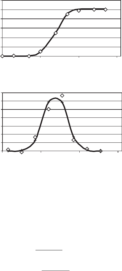
a sigmoidal response vs. either the dose or the logarithm of the dose (Figure 19.2a ).

That is, as dosage increases, the percent mortality will increase in a smooth, increasing

curve. The logarithm of the dose is often used, especially when the mean of the frequency

distribution is no more than two or three standard deviations above zero. This prevents the

theoretical problem of the distribution predicting toxic effects at negative dosages.

Each point on Figure 19.2a is the percent response, P

, at one dosage, d

. In the

Daphnia experiment example, this would be the result from one of the test tubes. If a

very large number of test tubes were tested covering a much larger number of different

dosages ðd

Þ, a histogr am could be prepared showing the frequency distribution for mor-

tality, called a tolerance distribution, TðdÞ. In typical toxicity tests there aren’t enough

dosage levels to do this. Instead, Tðd Þ can be estimated by numeri cally differentiating the

dose–response curve, PðdÞ, using successive pairs of points ðP

; d

Þ, ðP

iþ1

; d

iþ1

Þ, plotted at

the midpoint of each pair:

þ d

iþ1

’

iþ1

 P

iþ1

 d

ð19:1Þ

A sigmoidal dose–response curve would result in a bell-shaped tolerance distribution

as a function of dose. This leads naturally to an assumption of the normal distribution for

the shape of TðdÞ (Figure 19.2b). If this is a valid assumption, the dose–response curve

will be given by the integral of the normal distribution:

PðdÞ¼

1

ﬃﬃﬃﬃﬃﬃ

exp

u



du Y ¼ a þbx ð19:2Þ

where x is either the dose, d, or the logarithm of the dose, as described above. The dis-

tribution has two para meters, a and b, related to the mean, d

mean

, and standard deviation,

772 DOSE–RESPONSE RELATIONSHIPS

s, of the tolerance distribution. Several methods are available for estimat ing them. They

could be computed directly from the points of TðdÞ computed using the method of

moments. The procedure is as follows. First, equation (19.1) is used to compute TðdÞ.

Then the following equations are used to compute the mean and standard deviation:

mean

Tðd

ð19:3Þ

s ¼

ﬃﬃﬃﬃﬃﬃﬃﬃﬃﬃﬃﬃﬃﬃﬃﬃﬃﬃﬃﬃﬃﬃﬃﬃﬃﬃﬃﬃﬃﬃﬃﬃﬃﬃﬃﬃﬃﬃ

Tðd

 d

mean

ð19:4Þ

Several regression methods are also available, including nonlinear regression and maxi-

mum likelihood estimation. These have the advantage of producing not only the para-

meters but also a conﬁdence interval for the dose–response curve predicted. The

disadvantage of all the foregoing methods is that they may produc e poor results if the

data are not normally distributed or if the data do not cover the range of toxic effects

well. That is, the data must include at least one dosage with essentially zero response

and one with about 100% response. For example, if a bioassay on a wastewater produces

30% mortality at 100% concentration, these methods will not work.

100

120

140

01 2 3

100

120

0123

Dose-response curve

Percent mortality

Log dose

dose

Slope of response

Toxicity distribution

(a)

(b)

Figure 19.2 ðaÞ Sigmoidal logarithmic dose–response relationship; ðbÞ normal tolerance

distribution of mortality frequency.

TOLERANCE DISTRIBUTIO N AND DOSE–RESPONSE RELATIO NSHIPS 773

There are several procedures, called nonparametric methods, that do not make dis-

tributional assumptions. One of thes e is the trimmed Spearman–Kar ber method, which is a

numerical procedure for estimating the centroid of the tolerance distribution. Another is

the binomi al conﬁdence interval, which is used when the data do not include partial kills.

The nonparametric methods, however, often cannot estimate the standard deviation of the

tolerance distribution.

The d

mean

corresponds to the dose at which half of an exposed population would be

expected to suffer the effect. This is called the median lethal dose ðLD

Þ or median

effective dose ðED

Þ. Of course, LD, refers only to results of tests where the measured

response is mortality; ED, on the other hand, can be based on any toxicological effect. If

the dose is measured in concentration units, the median may be refered to as lethal con-

centration ðLC

Þ or effective concentration ðEC

Þ instead. If the effect is reduction in

growth rate, as commonly applied to microorganisms, a parameter known as the medi an

inhibitory concentration ðIC

Þ may be used. This is the concentration that would reduce

the growth rate by 50%. These parameters are commonly used as a basi s to compare the

toxicity of various toxic agents. A common qualitative classiﬁcation of LD

is given in

Table 19.2. Keep in mind that although only 50% may experience mortality at a given

dosage, it is likely that all the organisms will suffer deleterious toxicological effects

but that some may recover or at least survive. In the following discussion of toxicity,

we will refer to LD

, although the same principles apply to the other measures of median

effect.

Of course, it must be noted that the LD

is a property not only of the toxic agent but

also of experimental variables such as the organism, the time scale of the test, the method

of dosing, and so on. One can also refer to other percentiles, such as the lethal dose that

causes 1% or 10% mortality, the LD

or LD

, respectively.

The standard deviation, s, is related to the ‘‘steepness’’ of the dose–response relation-

ship. A steep slope indicates that the organism responds strongly to increases in dosage. A

ﬂatter response curve can be caused by slow absorption, rapid excretion or detoxiﬁcation,

or delayed bioactivation. In a normal distribution, 68.3% of the population will be within

one standard deviation of the mean, 95.5% within two, and so on. Table 19.3 summarizes

the relationship. Precise standard deviations are given for several of the percentiles of

interest (e.g., 1% and 10%). These can be used to compute LD

and LD

from s and

, keeping in mind that the standard deviation is computed in log- transformed units:

¼ LD

 10

2:326 s

ð19:5Þ

¼ LD

 10

1:282 s

ð19:6Þ

TABLE 19.2 Qualitative Classiﬁcation of Toxic Compounds

Classiﬁcation LD

Range (mg/kg) Example LD

of Example

Supertoxic 5 or less Dioxin in guinea pig 0.002

Extremely toxic 5–50 Parathion in goats 42

Highly toxic 50–500 DDT in rat 100

Moderately toxic 500–5,000 Strychnine in rat 2,000

Slightly toxic 5,000–15,000 Ethanol in mouse 10,000

Practically nontoxic > 15,000

774

DOSE–RESPONSE RELATIONSHIPS

Thus, you should be able to see that two compounds could have the same LD

, but if

one has a larger value of s (a less steep dose–response curve), its LD

and LD

will be

lower. This has important consequences for the use of toxicological data in environmental

applications. A mortality of 50% woul d be far too high to be tolerated in real life. How-

ever, handbooks often report only the LD

. Thus, the potential exists to greatly overes-

timate, or worse, underestimate the relative toxicity of a compound. Thus, it would be

useful for slope information or lower percentile LD values to be given also. However,

these data are not commonly available. Note, on the other hand, that because the dose–

response relationship is ﬂatter near the LD

or LD

, the uncertainty in their values will

be much greater than for LD

Example 19.1 Table 19.4 contains hypothetical results from an aquatic bioassay on the

toxicity of wastewater to Daphnia. The ﬁrst column, d, is the dosage as the percentage of

wastewater in the solution to which the Daphnia were exposed. The second column, n,is

the total number of organisms tested at each dosage; the third column, m, is the number

killed after 48 hours of exposure; and M is the percent morta lity, m=n. Since the control

ðd ¼ 0%Þ shows 4.7% mortality, we should ﬁrst decrease both n and m by 4.7% of m. The

ratio of the resulting numbers is the adjusted percent mortality, M

. A plot of M

versus d

gives the dose–response curve shown in Figur e 19.2 a .

TABLE 19.3 Normal Distribution and the Relation to Probits

Standard Deviations Cumulative

from the Mean Probits Percentage

3 2 0.14

2 3 2.28

1 4 15.9

0 5 50.0

1 6 84.1

2 7 97.7

3 8 99.87

3.090 1.910 0.10

2.326 2.674 1.00

1.282 3.718 10.0

0.674 4.326 25.0

TABLE 19.4 Hypothetical Aquatic Bioassay Results and Tolerance Distribution Analysis

dnmMMdTðdÞ d  Td

 T

0% 43 2 4.7% 0.0% 20% 0.103 0.021 0.004

40% 35 3 8.6% 4.1% 45% 1.309 0.589 0.265

50% 38 8 21.1% 17.2% 55% 2.877 1.582 0.870

60% 33 16 48.5% 46.0% 65% 1.994 1.296 0.843

70% 40 27 67.5% 65.9% 75% 2.305 1.728 1.296

80% 38 34 89.5% 89.0% 85% 0.521 0.443 0.377

90% 36 34 94.4% 94.2% 95% 0.265 0.252 0.239

100% 33 32 97.0% 96.8% 9.374 5.911 3.894

TOLERANCE DISTRIBUTIO N AND DOSE–RESPONSE RELATIO NSHIPS 775

From the data we can see that 50% mortality falls between dosages of 60 and 70%. By

interpolating linearly between these two points, we can estimate LC

as 62.0%. Simi-

larly, LC

falls between 40 and 50% concentration, and by interpolation we ﬁnd LC

to be 44.5%. However, we would expect the latter value to be too high, because the

response curve in this region will be curved upward. Better accuracy can be obtained

using the method of moments. First, it is necessary to compute the tolerance distribution

using equation (19.1). This gives the results shown in the sixth and seventh columns of

Table 19.4 [d and TðdÞ] and plotted in Figure 19.2b. Note that the dosages correspond to

the midpoints between those in the ﬁrst column.

Equations (19.2) and (19.3) require the sums of T, dT, and d

T. These values are

tabulated in the last three colu mns of Table 19.4, and the sums are the numbers in the

bottom row. Thus, the mean of the distribution is d

mean

¼ 5:911=9:374 ¼ 63:1%, and

s ¼ð3:894=9:374  0:631

1=2

¼ 13:3%. Thus, LC

¼ 63:1%, and from equations

(19.5) and (19.6), LC

¼ 42:6 and LC

¼ 30:9 %. You can see that in this case, the inter-

polation estimates of LC

and LC

were not far off and that the LC

was overestimated,

as expected. The curves in Figure 19.2a and b are the normal distribution with the mean

and standard deviation from this example.

Toxicology retains a curious legacy from precomputer days. To simplify hand calcula-

tions involving the normal distribution, toxicologists avoided the use of negative numbers

by the expedient of adding an arbitrary value of 5 to the standard deviations. The resulting

units are called probits. Thus, 2 standard deviations from the mean is the same as þ3

probits (see Table 19.3). The median, or LD

(0 standard deviations) becomes 5 probits.

This has become standard practice and remains in use today.

The assumption that the tolerance distribution is normal is not based on fundamental

principles, and a number of other distributions have been proposed. The best known is the

logit, in which the following equation replaces equat ion (19.2):

P ¼

1 þ e

ð19:7Þ

Another is the logistic function, which is based on hit theory (described in the next

section):

P ¼

1 þ e

ðaþbxÞ

ð19:8Þ

These models have advantages over the probit model in that the parameters of the logit

model can be estimated by linear least-squares methods, and the logistic equation has a

mechanistic basis. However, the probit or log-probit model is more established. The prac-

tical differences between these models are not very great, and their selection is often a

matter of personal preference and custom.

19.2 MECHANISTIC DOSE –RESPONSE MODELS

These models developed from hit theory explanations for carcinogenesis, and cancer

remains their most important application. The one-hit model (originally developed for

radiation effects) ﬁts the assumption that a single reaction event can transform a cell to

776 DOSE–RESPONSE RELATIONSHIPS

produce the toxic effect, and that the probability of a hit occurring is proportional to the

dosage:

PðdÞ¼1  expðbdÞ b > 0 ð19:9Þ

However, the one-hit model did not ﬁt data well. A multihit model improved this situation.

It assumed that several hits were necessary for a toxic effect, all of which had the same

probability. This led to the multistage model, to ﬁt the theory of carcinogenesis, which

requires several hits to the same cell, each having different probabilities, to produce a

malignancy:

PðdÞ¼1  exp 

i¼1

 0 ð19:10Þ

The parameter k is the number of stages. Although evidence may indicate many stages

(e.g., ﬁve stages in the case of colon cancer described above), for statistical validity

at least k þ 1 different dosage levels must be tested to determine k coefﬁcients. It is

often cost prohibitive to have so many levels. Note that dosage in these models is not

log-transformed, as is often done in the probit model.

Both of these models approach linearity as dose goes to zero. However, when equation

(19.10) is extrapolat ed to doses far below those used in the calculation, the uncertainty

becomes large. This is handled by replacing the linear term in equation (19.10)

(the term with i ¼ 1) with its upper 95% conﬁdence limit. This results in the linearized

multistage model, which is the preferred model in use by the U.S. EPA for carcinogenesis.

All of these models are linear in the low-concentration range. However, the one-hit

model cannot describe a sigmoidal curve. The multistage model can, and has the further

advantage over the probit or normal distribution model that it can describe asymmetric

tolerance distributions.

19.3 BACKGROUN D RESPONSE

For the probit model any toxic response in zero dosage control is usually subtracted from

all the data. Thus, what is used in the calculations is the excess mortality or toxic effect.

For stochastic biological models, where a hit can be caused by natural background causes,

the response can be adjusted for the probability of that o ccurring. In this case, PðdÞ is

interpreted as the additional risk over background, which can be attributed to the dose d:

PðdÞ¼



ðdÞp

1  p

ð19:11Þ

where P



ðdÞ is the observed response and p is the probability of a spontaneous hit. The

value of p may be so small that it cannot be measured directly in laboratory animals. In

such a case, it could be estimated by extrapolating dose–response data to zero dose, as

described in the next section.

19.3.1 Low-Dose Extrapolation

For many toxic effects, especially carcinogenesis, the goal is to control environmental

exposures to keep the risk at an extremely low level. A typical regulatory goal for a

BACKGROUND RESPONSE 777