Velten K. Mathematical Modeling and Simulation: Introduction for Scientists and Engineers
Подождите немного. Документ загружается.

2.5 Neural Networks 95
is this:
Eigenvalues of the Hessian:
362646.5 2397.25 16.52111
1.053426 0.01203984 0.003230483
0.00054226 0.0004922841 0.0003875433
0.0001999698 7.053957e-05
(2.75)
Since all eigenvalues are positive, we can conclude here that this particular neural
network corresponds to a secure local minimum of RSQ.
2.5.5
Generalization and Overfitting
The decay parameter of the nnet command remains to be discussed. In
NNetEx1.r, decay=1e-4 was used (line 5 of program 2.73). If you set decay=0
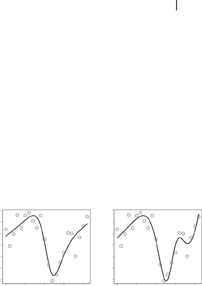
instead, you can obtain results such as the one shown in Figure 2.11a. Comparing
this with Figure 2.10, you see that this fits the data much better, which is also
reflected by an improved RSQ value (RSQ = 45.48 in Figure 2.11a compared to
RSQ = 103.4 in Figure 2.10). Does this mean that the best results are obtained
for
decay=0? To answer this question, let us increase the size of the hidden layer.
Until now,
size=3 was used in all computations, that is, a hidden layer comprising
of three nodes. Increasing this parameter, we increase the number of weights and
biases that can be tuned toward a better fit of the neural network and the data, and
hence we increase the flexibility of the neural network in this way. Figure 2.11b
shows a result obtained for a hidden layer with nine nodes (
size=9). In terms of
(a) (b)
6
4
2
0
−2
−4
−6
1920 1925 1930 1935 1940
Year
6
4
2
0
−2
−4
−6
I
I
1920 1925 1930 1935 194
0
Year
Fig. 2.11 Illustration of overfitting: results of NNEx1.r using
(a)
decay=0 and size=3 (b) decay=0 and size=9.

96 2 Phenomenological Models
the RSQ, this neural network is again better than the previous one (RSQ = 30.88
in Figure 2.11b compared to RSQ = 45.48 in Figure 2.11a). Obviously, this im-
provement is achieved by the fact that the neural network in Figure 2.11b follows
an extra curve compared to the network in Figure 2.11a, attempting to ‘‘catch’’ as
many data points as possible as closely as possible.
This behavior is usually not desired since it restricts the predictive capability of a
neural network. Usually, one wants neural networks to have the following
Definition 2.5.1 (Generalization property) Suppose two mathematical models
(S, Q, M)and(S, Q, M
∗
) have been setup using a training dataset D
train
.Then
(S, Q, M)issaidtogeneralize better than (S, Q, M
∗
)onatest dataset D
test
with
respect to some error criterion E,if(S, Q, M) produces a smaller value of E on
D
test
compared to (S, Q, M
∗
).
You may think of (S, Q, M)and(S, Q, M
∗
) as being regression or neural network
models, and of E as being the RSQ as discussed above. Note that the mathematical
models compared in Definition 2.5.1 refer to the same system S and to the same
question Q since the generalization property pertains to the ‘‘mathematical part’’
of a mathematical model. The definition emphasizes the fact that it is not sufficient
to look at a mathematical model’s performance on the dataset which was used to
construct the model if you want to achieve good predictive capabilities (compare the
discussion of cross-validation in Section 2.3.3). To evaluate the predictive capabili-
ties, we must of course look at the performance of the model on datasets that were
not used to setup the model, and this means that we must ask for the generalization
property of a model. Usually, better predictions are obtained from mathematical
models which describe the essential tendency of the data (such as the neural net-
works in Figures 2.10 and 2.11a) instead of following random oscillations in the data
similar to Figure 2.11b. The phenomenon of a neural network fitting the data so
‘‘well’’ that it follows random oscillations in the data instead of describing the gen-
eral tendency of the data is known as overfitting [45]. Generally, overfitting is related
with an increased ‘‘roughness’’ of the neural network function, since overfitted neu-
ral networks follow extra curves in an attempt to catch as many data points as possi-
ble as described above. The overfitting phenomenon can be defined as follows [66]:
Definition 2.5.2 (Overfitting) Amathematicalmodel(S, Q, M)issaidtooverfit
a training dataset D
train
with respect to an error criterion E and a test dataset
D
test
,ifanothermodel(S, Q, M
∗
) with a larger error on D
train
generalizes better
to D
test
.
For example, the neural network model behind Figure 2.11b will overfit the
training data in the sense of the definition if it generates a larger error on unknown
data e.g. compared to the neural network model behind Figure 2.10.
There are several strategies that can be used to reduce overfitting [45, 64]. So-called
regularization methods use modified fitting criteria that penalize the ‘‘roughness’’

2.5 Neural Networks 97
of the neural network, which means that these fitting criteria consider for example,
both the RSQ and the roughness of the neural network. In terms of such a modified
fitting criterion, a network such as the one in Figure 2.11a can be better than the
‘‘rougher’’ network in Figure 2.11b (although the RSQ of the second network is
smaller). One of these regularizations methods called weight decay makes use of the
fact that the roughness of neural networks is usually associated with ‘‘large’’ values
of its weight parameters, and this is why this method includes the sum of squares of
the network weights in the fitting criterion. This is the role of the
decay parameter
of the
nnet command: decay=0 means there is no penalty for large weights in the
fitting criterion. Increasing the value of
decay, you increase the penalty for large
weights in the fitting criterion. Hence
decay=0 means that you may get overfitting
for neural networks with sufficiently many nodes in their hidden layer, while
positive values of the
decay parameter decrease the ‘‘roughness’’ of the neural
network and will generally improve its predictive capability. Ripley suggests to use
decay values between 10
−4
and 10
−2
[67, 68]. To see the effect of this parameter,
you may use a hidden layer with nine nodes similar to Figure 2.11b, but with
decay=1e-4. Using these settings, you will observe that the result will look similar
to Figures 2.10 and 2.11a, which means you get a much smoother (less ‘‘rough’’)
neural network compared to the one in Figure 2.11b.
2.5.6
Several Inputs Example
As a second example which involves several input quantities, we consider the data
in
rock.csv which you find in the book software. These data are part of the R
package, and they are concerned with petroleum reservoir exploration. To get oil out
of the pores of oil-bearing rocks, petroleum engineers need to initiate a flow of the
oil through the pores of the rock toward the exploration site. Naturally, such a flow
consumes more or less energy depending on the overall flow resistance of the rock,
and this is why engineers are interested in a prediction of flow resistance depending
on the rock material. The file
rock.csv contains data that were obtained from
48 rock sample cross-sections, and it relates geometrical parameters of the rock
pores with its permeability, which characterizes the ease of flow through a porous
material [69]. The geometrical parameters in
rock.csv are: area,ameasureof
the total pore spaces in the sample (expressed in pixels in a 256 × 256 image);
peri, the total perimeter of the pores in the sample (again expressed in pixels);
and
shape, a measure of the average ‘‘roundness’’ of the pores (computed as the
smallest perimeter divided by the square root of the area for each individual pore;
approx. 1.1 for an ideal circular pore, smaller for noncircular shapes). Depending
on these geometrical parameters,
rock.csv reports the rock permeability perm
expressed in units of milli Darcy (= 10
−3
Darcy, see [70]).
In a first attempt to describe these data using a neural network, let us consider
two explanatory variables,
area and peri, neglecting the third geometrical variable,
shape. With this restriction we will be able to generate 3D graphical plots of the
neural network below. Moreover, we will take
log(perm) as the response variable
98 2 Phenomenological Models
since perm covers several orders of magnitude (see rock.csv). Note that within
R,
log denotes the natural logarithm. To compute the neural network, we can
proceed as above and start e.g. with
NNEx1.r, editing the model and the name of
the data file. This has been done in the R program
NNEx2.r which you find in
the book software. The core of the code in
NNEx2.r that does the neural network
computing is very similar to program 2.73 above. Basically, we just have to replace
line1of2.73with
eq=log(perm)~area+peri
(2.76)
Again, a scaling of the explanatory variables must be applied similar to the one
in line 4 of program 2.73 (see Note 2.5.4), but we leave out these technicalities here
(see
NNEx2.r for details). If you run NNex2.r within R, you will get results similar
to the one shown in Figure 2.12 (note that you may obtain slightly different results
for the reasons explained in the discussion of
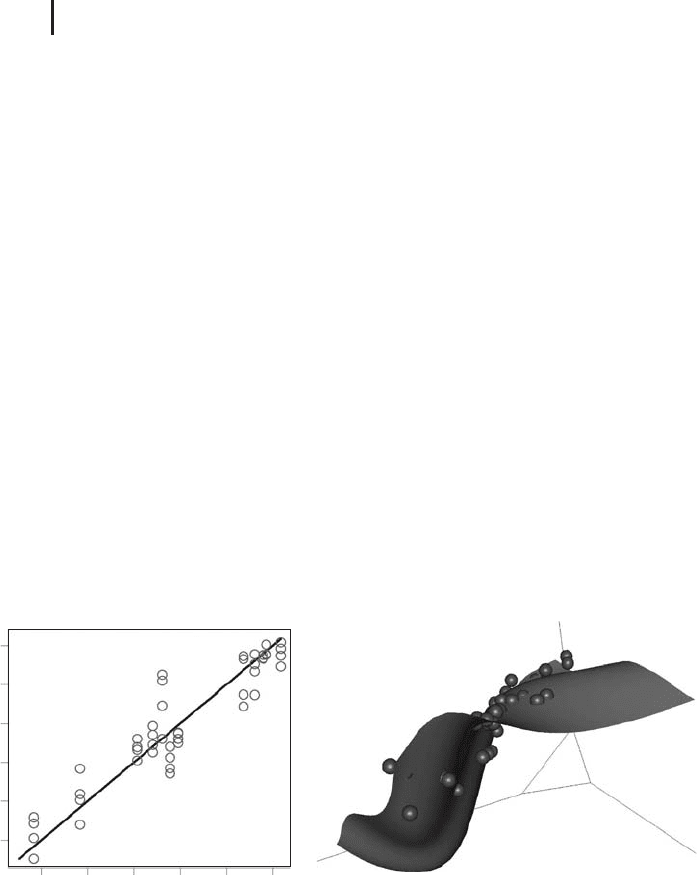
NNEx1.r). Figure 2.12 compares the
neural network with the data in a way similar to the one in Section 2.4 above, using
a predicted-measured plot and a conventional 3D plot. The 3D plot shows how
the neural network builds up a nonlinear, three-dimensional surface that attains
a shape that follows the essential tendency in the data much better than what
could be achieved by multiple regression (note that in this case multiple regression
amounts to fitting a flat surface to the data). This is also reflected by the residual
sums of squares computed by
NNex2.r: RSQ = 32.7 in the multiple linear model,
and RSQ = 15 for the neural network model.
7
6
5
4
3
2
Perm (predicted)
234567
Perm (measured)
area
[pix
2
]
peri
[pix]
perm [mD]
(a) (b)
Fig. 2.12 Comparison of a neural network predicting perm
depending on area and peri with the data in rock.csv
(a) in a predicted-measured plot and (b) in a conventional
plot in the
area-peri-perm 3d-space. Plots generated by
NNEx2.r.

2.6 Design of Experiments 99
Until now we have left out the shape variable of rock.csv as an explanatory
variable. Changing the model within
NNEx2.r to
eq=log(perm)~area+peri+shape
(2.77)
a neural network involving the three explanatory variables area, peri and shape is
obtained, and in this way fits with an even better RSQ around 10 can be obtained.
Similar to
NNEx1.r, NNEx2.r plots the eigenvalues of the Hessian matrix so that
you can check if a secure local minimum of the fitting criterion has been achieved
as discussed above (e.g. Figure 2.12 refers to a neural network which has positive
eigenvalues of the Hessian only as required). Finally, you should note that to
evaluate the predictive capabilities of the neural networks discussed in this section,
cross-validation can be used similar to above (Section 2.3.3).
Neural networks are useful not only for prediction, but also to visualize and better
understand a dataset. For example, it can be difficult to understand the effects of
two explanatory variables on a dependent variable (e.g. the effects of
area and
peri on perm in the above example) based on a 3D scatterplot of the data (the
spheres in Figure 2.12b) only. In this case, a three-dimensional nonlinear neural
network surface that approximates the data similar to Figure 2.12b can help us to
see the general nonlinear form described by the data. Of course, linear or nonlinear
regression plots such as Figure 2.8 can be used in a similar way to visualize
datasets.
Note 2.5.7 (Visualization of datasets) Neural networks (and mathematical
models in general) can be used to visualize datasets. An example is Figure 2.12b,
where the model surface highlights and accentuates the nonlinear effects of two
explanatory variables on a dependent variable.
2.6
Design of Experiments
Suppose you want to perform an experiment to see if there are any differences in
the durability of two house paintings A and B. In an appropriate experiment, you
would e.g. paint five wall areas using paint A and five other wall areas using paint
B. Then, you would measure the durability of the paintings in some suitable way,
for example, by counting the number of defects per surface area after some time.
The data could then be analyzed using the t test (Section 2.1). This example is
discussed in [71], and the authors comment on it as follows:
You only have to paint a house once to realize the importance of this experi-
ment.

100 2 Phenomenological Models
Since the time and effort caused by an experiment as well as the significance of
its results depend very much on an appropriate design of the experiment, this can
also be phrased as follows:
Note 2.6.1 (Importance of experimental design) You only have to paint a house
once to realize the importance of an appropriate design of experiments.
Indeed, the design of experiments – often abbreviated as DOE –isanimportant
statistical discipline. It encompasses a great number of phenomenological models
which all focus on an increase of the efficiency and significance of experiments. Only
a few basic concepts can be treated within the scope of this book, and the emphasis
will be on the practical software-based use of these methods. The reader should
refer to books such as [41, 72, 73] to learn about more advanced topics in this field.
2.6.1
Completely Randomized Design
Figure 2.13 shows a possible experimental design that could be used in the house
painting example. The figure shows 10 square test surfaces on a wall which are
labeled according to the paint (A or B) that was applied on each of these test
surfaces. This is a ‘‘naive’’ experimental design in the sense that it reflects the first
thought which many of us may have when we think about a possible organization
ofthesetestsurfaces.And,asitisthecasewithmanyofour‘‘firstthoughts’’in
many fields, this is a bad experimental design, even the worst one imaginable.
The point is that most experiments that are performed in practice are affected by
nuisance factors which, in many cases, are unknown and out of the control of the
experimenter at the time when the experiment is designed. A great number of such
possible nuisance factors may affect the wall painting experiment. For example,
there may be two different rooms of a house behind the left (‘‘A’’) and right (‘‘B’’)
halves of the wall shown in Figure 2.13, and the temperature of one of these rooms
and, consequently, the temperature of one half of the wall may be substantially
higher compared to the temperature of the other room and the other half of the
wall. Since temperature may affect the durability of the painting, any conclusions
drawn from such an experiment may hence be wrong.
This kind of error can very easily be avoided by what is called a completely
randomized design or CRD design. As the name suggests, a completely randomized
design is a design where the positions of the A and B test surfaces are determined
Fig. 2.13 House painting example: naive experimental de-
sign, showing a wall (large rectangle) with several test sur-
faces which are painted using paints A or B.

2.6 Design of Experiments 101
randomly. Based on the usual technical terminology, this can be phrased as
follows: A completely randomized design is a design where the treatments or
levels (corresponding to A and B in this case) of the factor under investigation
(corresponding to the paint) are assigned randomly to the experimental units
(corresponding to the test surfaces).
Using software, this can be done very easily. For example, Calc’s
rand() function
can be used as follows (see Section 2.1.1 and Appendix A for details about Calc):
Completely randomized design using Calc
•
Generate a Calc spreadsheet with three columns labeled as
Experimental unit, Random number and Factor level
•
Write the desired factor levels in the Factor level column, for
example, ‘‘A’’ in five cells of that column and ‘‘B’’ in another five
cells in the case of the wall painting example.
•
Enter the command =rand() in the cells of the Random number
column (of course, it suffices to enter this into the top of that
column, which can then be copied to the other cells using the
mouse – see Calc’s help pages for details).
•
Use Calc’s ‘‘Data/Sort’’ menu option to sort the data with respect
to the Random number column.
•
Write 1, 2, 3, ... in the Experimental unit column of the
spreadsheet, corresponding to an enumeration of the
experimental units that was determined before this procedure
was started.
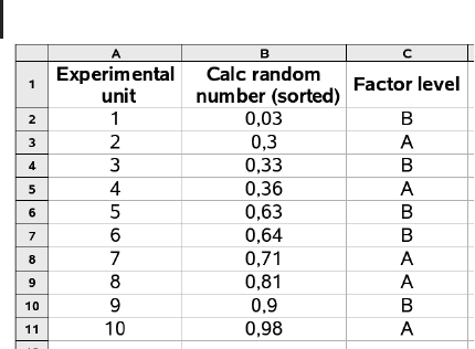
In the wall painting example, this procedure yields e.g. the result shown in
Figure 2.14, which defines a random assignment of the test surfaces (which we can
think of as being enumerated from 1 to 10 as we move from the left to the right
side of the wall in Figure 2.13) to the factor levels A and B. Figure 2.14 has been
generated using the Calc file
CRD.ods in the book software (see Appendix A). Note
that when you generate your own completely randomized designs using this file,
you will have to enter the
rand() command into the cells of the Random number
column of that file again.
Assuming a higher temperature of the left part of the wall in Figure 2.13 as
discussed above, this higher temperature would affect both the A and B test
surfaces based on the completely randomized design in Figure 2.14. Hence,
although the results still would be affected by the temperature variation along the
wall since the variance of the data would be higher compared to an isothermal
experiment, the completely randomized design would at least prevent us from
wrong conclusions caused by the fact that the higher temperatures would be
attributed to one of the factor levels only as discussed above.
A completely randomized design can also be generated using the
design.crd
function which is a part of R’s agricolae package. For the house painting example,
102 2 Phenomenological Models
Fig. 2.14 Completely randomized design for the house paint-
ing example, computed using Calc’s
rand() function. See
the file
CRD.ods in the book software.
thiscanbedoneusingthefollowingcode(seeCRD.r in the book software):
1: library(agricolae)
2: levels=c("A", "B")
3: rep=c(5,5)
4: out=design.crd(levels,rep,number=1)
5: print(out)
(2.78)
After the agricolae package is loaded in line 1, the levels (A and B in the
above example) and the number of replications of each level (5 replications for A
and B) are defined in the variables
levels and rep, which are then used in the
design.crd command in line 4 to generate the completely randomized design.
Thedesignisthenstoredinthevariable
out, which is printed to the screen using
R’s
print command in line 5. The result may look like this (may: depending on
the options that you choose for random number generation, see below):
plots levels r plots levels r
11A1 66B3
22B1 77B4
33A2 88A4
44B2 99A5
5 5 A 3 10 10 B 5
Here, the ‘‘plots’’ and ‘‘levels’’ columns correspond to the ‘‘Experimental
unit’’ and ‘‘Factor level’’ column in Figure 2.14, while the ‘‘
r’’ column counts
the number of replications separately for each of the factor levels. Note that the
result depends on the method that generates the random numbers that are used
to randomize the design. A number of such methods can be used within the
agricolae package (see the documentation of this package).

2.6 Design of Experiments 103
2.6.2
Randomized Complete Block Design
Consider the following experiment that is described in [72]: A hardness testing
machine presses a rod with a pointed tip into a metal specimen with a known
force. The depth of the depression caused by the tip is then used to characterize
the hardness of the specimen. Now suppose that four different tips are used in
the hardness testing machine and that it is suspected that the hardness readings
depend on the particular tip that is used. To test this hypothesis, each of the four
tips is used four times to determine the hardness of identical metal test coupons.
In a first approach, one could proceed similar to the previous section. The hardness
experiment involves one factor (the tip), four levels of the factor (tip 1–tip 4),
and four replications of the experiment at each of the factor levels. Based on this
information, a completely randomized design could be defined using the methods
described above.
However, there is a problem with this approach. Sixteen different metal test
coupons would be used in such a completely randomized design. Now it is possible
that these metal test coupons differ slightly in their hardness. For example, these
metal coupons may come from long metal strips, and temperature variations
during the manufacturing of these strips may result in a nonconstant hardness
of the strips and hence of the metal coupons. These hardness variations would
then potentially affect the comparison of the four tips in a completely randomized
experiment.
To remove the effects of possible hardness variations among the metal coupons,
a design can be used that uses only four metal test coupons and that tests each of
the four tips on each of these four test coupons. This is called a blocked experimental
design, since it involves four ‘‘blocks’’ (corresponding to the four metal test coupons)
where all levels of the factor (tip 1–tip 4) are tested in each of these blocks. Such
blocked designs are used in many situations in order to achieve more homogeneous
experimental units on which to compare the factor levels. Within the blocks, the
order in which the factor levels are tested should be chosen randomly for the same
reasons that were discussed in the previous section, and this leads to what is called
a randomized complete block design (RCBD).
In R, a RCBD for the above example can be computed using the following code
(see
RCBD.r in the book software):
1: library(agricolae)
2: levels=c("Tip 1", "Tip 2", "Tip 3", "Tip 4")
3: out=design.rcbd(levels,4,number=1)
5: print(out)
(2.79)
This code is very similar to the code 2.78 above, except for the fact that the
command
design.rcbd is used here instead of design.crd. Note that the sec-
ond argument of
design.rcbd gives the number of blocks (4 in this case). The
code 2.79 may yield the following result in R (may: see the above discussion of
104 2 Phenomenological Models
Equation 2.78):
plots block levels plots block levels
1 1 1 Tip 2 9 9 3 Tip 3
2 2 1 Tip 1 10 10 3 Tip 2
3 3 1 Tip 4 11 11 3 Tip 4
4 4 1 Tip 3 12 12 3 Tip 1
5 5 2 Tip 1 13 13 4 Tip 2
6 6 2 Tip 3 14 14 4 Tip 4
7 7 2 Tip 4 15 15 4 Tip 3
8 8 2 Tip 2 16 16 4 Tip 1
This result can be interpreted similar to the corresponding result of design.crd
that was discussed in the previous section. Again, the ‘‘plots’’ column just counts
the experiments, the ‘‘
block’’ column identifies one of the four blocks correspond-
ing to the four metal test coupons, and the ‘‘
levels’’ column prescribes the factor
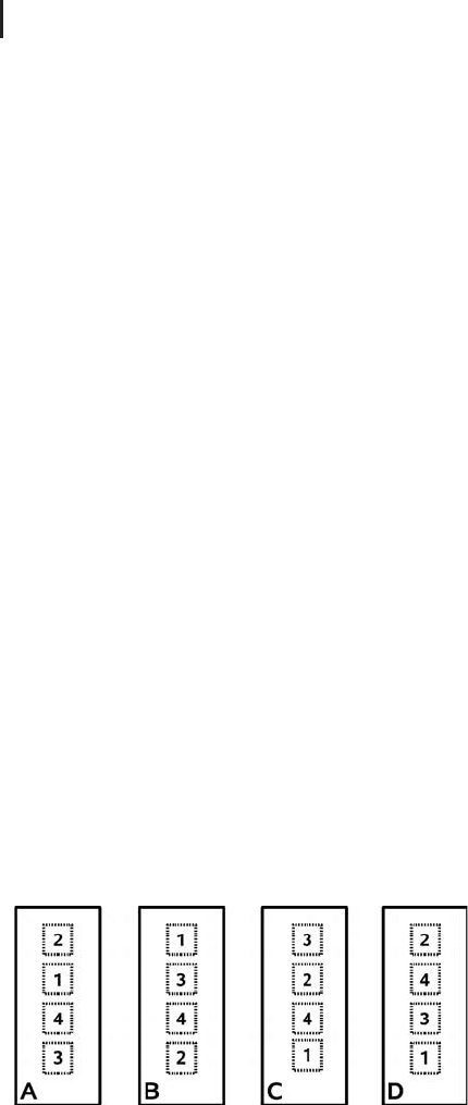
level to be used in each experiment. Figure 2.15 visualizes this experimental design.
Note that each of the tips is used exactly once on each of the metal test coupons as
required.
2.6.3
Latin Square and More Advanced Designs
Again, there may be a problem with the experimental design described in the
last section. As Figure 2.15 shows, tip 4 is tested three times in the third run
of the experiment that is performed on the metal test coupons A–C. Now it
may very well be that the result of the hardness measurement depends on the
number of hardness measurements that have already been performed on the same
test coupon. Previous measurements that have been performed on the same test
coupon may have affected the structure and rigidity of the test coupon in some
way. To avoid this as much as possible, the experimenter may test the four tips on
different locations on the test coupon with a maximum distance between any two
Fig. 2.15 Randomized complete block design computed us-
ing
design.rcbd in R (hardness testing example): metal
test coupons A–D, and numbers indicating the randomly
chosen sequence of the tips 1–4.