Velten K. Mathematical Modeling and Simulation: Introduction for Scientists and Engineers

Подождите немного. Документ загружается.

2.2 Linear Regression 65

2.2

Linear Regression

Generally speaking, regression models involve the analysis of a dependent variable

in terms of one or several independent variables. In regression, the dependent

variable is expressed in terms of the independent variables using various types

of regression equations. Parameters in the regression equations are then tuned

in a way that ﬁts these equations to data. The idea of the regression method has

already been explained based on the spring data

spring.ods in Section 1.5. As

it was discussed there referring to the black box input–output system in Figure

1.8, one can say that regression is a really prototypical method among the existing

phenomenological modeling approaches. It contains all the essential ingredients:

an input x,anoutputy, a black box–type system transforming x into y,and

the attempt to ﬁnd a purely data-based mathematical description of the relation

between x and y.Thetermregression itself is due to a particular regression study

that was performed by Francis Galton who investigated human height data. He

found that, independent of their parents’ heights, the height of children tends to

regress toward the typical mean height [40].

2.2.1

The Linear Regression Problem

Assume we have a dataset (x

, y

), (x

, y

), ...,(x

, y

)(x

, y

∈ R , i = 1, ..., m,

m ∈ N). Then, the simplest thing one can do is to describe the data using a

regression function or model function of the form

y(x) = ax + b (2.27)

The coefﬁcients a and b in Equation 2.27 are called the regression coefﬁcients or the

parameters of the regression model. x is usually called the explanatory variable (or

predictor variable,orindependent variable), while

y (or y) is called the response variable

(or dependent variable). Note that the hat notation is used to distinguish between

measured values of the dependent variable (written without hat as y

)andvaluesof

the dependent variable computed using a regression function (which are written

in hat notation, see Equation 2.27). A function

y(x ) as in Equation 2.27 is called

a linear regression function since this function depends linearly on the regression

coefﬁcients, a and b [41].

Note 2.2.1 (Linear regression) A general one-dimensional linear regression

function

y(x ) computes the response variable y based on the explanatory vari-

able x and regression coefﬁcients a

, a

, ..., a

(s ∈ N). If the expression

y(x )

depends linearly on a

, a

, ..., a

, it can be ﬁtted to measurement data us-

ing linear regression. Higher-dimensional linear regression functions involving

multiple explanatory variables will be treated in Section 2.3, the nonlinear case

in Sections 2.4 and 2.5.

66 2 Phenomenological Models

Equation 2.27 ﬁts the data well if the differences y

−

y(x

)(i = 1, ..., m)are

small. To achieve this, let us deﬁne

RSQ =



i=1



−

y(x

)



(2.28)

This expression is called the residual sum of squares (RSQ). Note that RSQ

measures the distance between the data and the model: if RSQ is small, the

differences y

−

y(x

) will be small, and if RSQ is large, at least some of the

differences y

−

y(x

) will be large. This means that to achieve a small distance

between the data and the model, we need to make RSQ small. In regression, this

is achieved by an appropriate tuning of the parameters of the model. Precisely, the

parameters a and b are required to solve the following problem:

min

a,b∈R

RSQ (2.29)

Note that RSQ depends on a and b via

y. The solution of this problem can

be obtained by an application of the usual procedure for the minimization of a

function of several variables to the function RSQ(a, b) (setting the partial derivatives

of this function with respect to a and b to zero etc.) [17], which gives [19]

a =



i=1

− mx y



i=1

− mx

(2.30)

b =

y − ax (2.31)

The use of RSQ as a measure of the distance between the model and the data

may seem somewhat arbitrary since several other alternative expressions could

be used here (e.g. RSQ could be replaced by a sum of the absolute differences

−

y(x

)|). RSQ is used here since it leads to maximum likelihood estimates of the

model parameters, a and b, if one makes certain assumptions on the statistical

distribution of the error terms, y

−

y(x

) (see below). Using these assumptions, the

maximum likelihood estimates of the model parameters derived from minimizing

RSQ make the data ‘‘more likely’’ compared to other choices of the parameter

values [41].

2.2.2

Solution Using Software

Now let us see how this analysis can be performed using software. We refer

to the data in

spring.csv as an example again (see Section 1.5.6). Start the R

Commander asdescribedinAppendixBanthenimportthedata

spring.csv into

the R Commander using the menu option ‘‘Data/Import data/From text ﬁle’’. Then

choose the menu option ‘‘Statistics/Fit models/Linear regression’’ and select x and

y as the explanatory and response variables of the model, respectively. This gives

the result shown in Figure 2.2a.

2.2 Linear Regression 67

x(N)

2010 30 40 50

y(cm)

(a) (b)

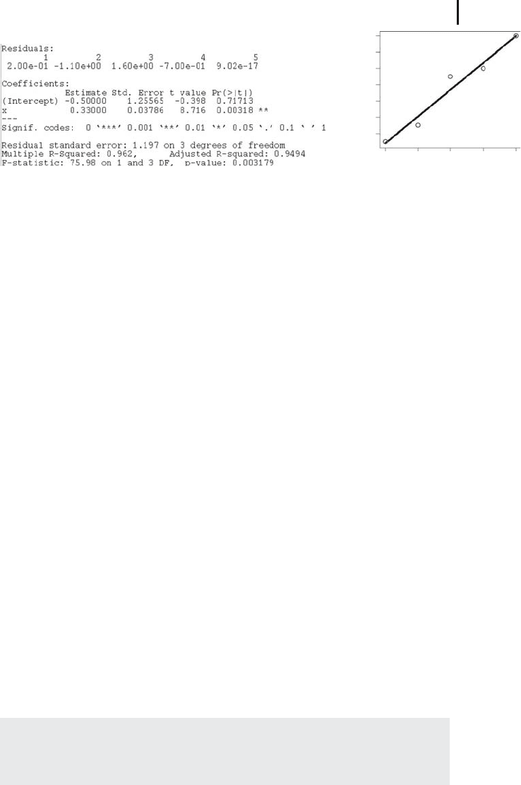
Fig. 2.2 (a) Linear regression result obtained using the R

Commander and the data in

spring.csv. (b) Compar-

ison of the regression line Equation 2.32 with the data

spring.csv.FigureproducedusingLinRegEx1.r.

The R output shown in Figure 2.2a ﬁrst reports the residuals between the data

and the model, that is, the differences y

−

y(x

)(i = 1, ..., m), which yields 5 values

in this case since

spring.csv contains 5 lines of data. You can get an idea about

the quality of the ﬁt between data and model based on these values, but it is of

course better to see this in a plot (see below). After this, R reports on the regression

coefﬁcients, in a table comprising two lines, the ﬁrst one (labeled

Intercept)

referring to the coefﬁcient b in Equation 2.27 and the second one (labeled

referring to the coefﬁcient a in the same equation. The labels used in this table are

justiﬁed by the fact that b describes the intercept of the line given by Equation 2.27,

that is, the position where this line crosses the y-axis, while a is the coefﬁcient that

multiplies the x in Equation 2.27. In the ‘‘

Estimate’’ column of Figure 2.2 you see

that a =−0.5andb = 0.33 have been obtained as the solution of Problem (2.29).

Using Equation 2.27, this means that we have obtained the following regression

line:

y(x) = 0.33x − 0.5 (2.32)

Figure 2.2b compares the regression line, Equation 2.32, with the data in

spring.csv. This ﬁgure has been generated using the R program LinRegEx1.r

in the book software. A similar ﬁgure can be produced using the R Commander

based on the menu option ‘‘Graphs/Scatterplot’’, but you should note that the R

Commander offers a limited number of graphical options only. Unlimited graphical

options (e.g. to change line thicknesses and colors) can be accessed if you are using

R programs such as

LinRegEx1.r. You will ﬁnd a few comments on the content

LinRegEx1.r further below in this section.

Note 2.2.2 (Regression coefﬁcients) Estimates of the regression coefﬁcients

in regression equations such as Equation 2.27 can be obtained using formulas

such as Equations 2.30 and 2.31, the R-Commander, or R programs such

68 2 Phenomenological Models

as LinRegEx1.r. Note that no formulas are available for general nonlinear

regression equations, as discussed in Section 2.4.

As Figure 2.2b shows, the regression line captures the tendency in the data. It is

thus reasonable to use the regression line for prediction, extrapolating the tendency

in the data using the regression line. Formally, this is done by inserting x values

into Equation 2.32. For example, to predict y for x = 60, we would compute as

follows:

y(60) = 0.33 ·60 − 0.5 = 19.3 (2.33)

Looking at the data in Figure 2.2b, you see that

y(60) = 19.3 indeed is a reasonable

extrapolation of the data. Of course, predictions of this kind can expected to be

useful only if the model ﬁts the data sufﬁciently well, and if the predictions are

computed ‘‘close to the data’’. For example, our results would be questionable if we

used Equation 2.32 to predict y for x = 600, since this x-value would be far away

from the data in

spring.csv. The requirement that predictions should be made

close to the data that have been used to construct the model applies very generally to

phenomenological models, including the phenomenological approaches discussed

in the next sections.

Note 2.2.3 (Prediction) Regression functions such as Equation 2.27 can be

used to predict values of the response variable for given values of the explanatory

variable(s). Good predictions can be expected only if the regression function ﬁts

the data sufﬁciently well, and if the given values of the explanatory variable lie

sufﬁciently close to the data.

2.2.3

The Coefﬁcient of Determination

As to the quality of the ﬁt between the model and the data, the simplest approach

is to look at appropriate graphical comparisons of the model with the data such

as Figure 2.2b. Based on that ﬁgure, you do not need to be a regression expert to

conclude that there is a good matching between model and data, and that reasonable

predictions can be expected using the regression line. A second approach is the

coefﬁcient of determination, which is denoted as R

. Roughly speaking, the

coefﬁcient of determination measures the quality of the ﬁt between the model and

the data on a scale between 0 and 100%, where 0% refers to very poor ﬁts and 100%

refers to a perfect matching between the model and the data. R

thus expresses the

quality of a regression model in terms of a single number, which is useful e.g. when

you want to compare the quality of several regression models, or if you evaluate

multiple linear regression models (Section 2.3) which involve higher-dimensional

regression functions

y(x

, x

, ..., x

) that cannot be plotted similar to Figure 2.2b

2.2 Linear Regression 69

(note that a plot of

y over x

, x

, ..., x

would involve an n + 1-dimensional space).

In the R-output shown in Figure 2.2a, R

is the Multiple R Squared value, and

hence you see that we have R

= 96.2% in the above example, which reﬂects the

good matching between the model and the data that can be seen in Figure 2.2b. The

Adjusted R Squared value in Figure 2.2a will be explained below in Section 2.3.

Formally, the coefﬁcient of determination is deﬁned as [37]



i=1



− y





i=1



− y



(2.34)

wherewehaveused

y(x

). For linear regression models, this can be rewritten as

= 1 −



i=1



−





i=1



− y



(2.35)

The latter expression is also known as the pseudo-R

and it is frequently used to

assess the quality of ﬁt in nonlinear models. Note that R

according to Equation 2.35

can attain negative values if the

values are not derived from a linear regression

(whereas Equation 2.34 guarantees R

> 0), and if these values are ‘‘far away’’

from the measurement values. If you observe negative R

values, then your model

performs worse than a model that would yield the mean value

y for every input

(i.e.

y(x

) = y, i = 1, ..., m), since such a mean value model would give R

= 0in

Equation 2.35.

In a linear model, it can be easily shown that R

expresses the ratio between the

variance of the predicted values (

, ...,

) and the variance of the measurement

values (y

, ..., y

). R

= 100% is thus usually expressed like this: ‘‘100% of the

variance of the measurement data is explained by the model.’’ On the other hand,

values substantially below 100% indicate that there is much more variance in

the measurement data compared to the model, and this means that the variance of

the data is insufﬁciently explained by the model, which means that one has to look

for additional explanatory variables. For example, if a very poor R

is obtained for a

linear model

y = ax + b, it may make sense to investigate multiple linear models

such as

y = ax + bz + c which involves an additional explanatory variable z (see

Section 2.3 below).

Note 2.2.4 (Coefﬁcient of determination) The coefﬁcient of determination, R

measures the quality of ﬁt between a linear regression model and data. On a scale

between 0 and 100%, it expresses how much of the variance of the dependent

variable measurements is explained by the explanatory variables of the model. If

is small, one can try to add more explanatory variables to the model (see the

multiple regression models in Section 2.3) or use nonlinear models (Sections 2.4

and 2.5).

70 2 Phenomenological Models

2.2.4

Interpretation of the Regression Coefﬁcients

You may wonder why the values of a and b appear in a column called Estimates in

the R output of Figure 2.2a, and why standard errors are reported for a and b in the

next column. Roughly speaking, this is a consequence of the fact that measurement

data typically are affected by measurement errors. For example, a measurement

device might exhibit a random variation in its last signiﬁcant digit, which might

lead to values such as 0.856, 0.854, 0.855, and 0.854 when we repeat a particular

measurement under the same conditions several times (beyond this, there may

be several other systematic and random sources of measurement errors, see [42]).

Now suppose that we analyze measurement data (x

, y

), (x

, y

), ...,(x

, y

)as

above using linear regression, which might lead us to regression coefﬁcients a and

b. If we repeat the measurement, the new data will (more or less) deviate from the

original data due to measurement errors, leading to (more or less) different values

of a and b in a regression analysis. The parameters a and b thus depend on the

random errors in the measurement data, and this means that a and b can be viewed

as realizations of random variables α and β (see Section 2.1.2.1).

Usually, it is assumed that these random variables generate the measurement

data (x

, y

), (x

, y

), ...,(x

, y

) as follows:

= αx

+ β + 

, i = 1, ..., m (2.36)

where the 

expresses the deviation between the model and the data, which

includes the measurement error. The error terms 

are typically assumed to be

normally distributed with zero expectation and a constant variance σ

independent

of i (so-called homoscedastic error terms). Using these assumptions, the standard

errors of α and β can be estimated, and these estimates are reported in the column

Std.Error of the R output in Figure 2.2a. As you see there, the standard error

of α is much smaller than the standard error of β, which means that you may

expect larger changes of the estimate of β compared to the estimate of α if you

would perform the same analysis again using a different dataset. In other words,

theestimateofβ is ‘‘less sharp’’ compared to that of α. The numbers reported

in the column ‘‘

t value’’ of Figure 2.2a refer to the Student’s t distribution, and

they can be used e.g. to construct conﬁdence intervals of the estimated regression

coefﬁcients as explained in [19]. The values in the last column of Figure 2.2a are

the p values that have been discussed in Sections 2.1.3.2 and 2.1.3.4.

2.2.5

Understanding

LinRegEx1.r

AbovewehaveusedtheR program LinRegEx1.r to produce Figure 2.2b. See

Appendix B for any details on how to use and run the R programs of the book

2.2 Linear Regression 71

software. The essential commands in this code can be summarized as follows:

1: eq=y~x

2: FileName="Spring.csv"

3: Dataset=read.table(FileName,

...)

4: RegModel=lm(eq,data=Dataset)

5: print(summary(RegModel))

6: a=10

7: b=50

8: xprog=seq(a, b, (b-a)/100)

9: yprog=predict(RegModel, data.frame(x = xprog))

10: plot(xprog,yprog,

...)

(2.37)

As mentioned before, the numbers ‘‘1:’’,‘‘2:’’, and so on in this code are not

a part of the program, but just line numbers that are used for referencing in our

discussion. Line 1 deﬁnes the regression equation in a special notation that you

ﬁnd explained in detail in R’s help pages and in [43]. The command in line 1 stores

the regression equation in a variable

eq whichisthenusedinline4tosetupthe

regression model, so

y∼x is the part of line 1 that deﬁnes the regression equation.

Basically,

y∼x can be viewed as a short notation for Equation 2.27, or for Equation

2.36 (it implies all the statistical assumptions expressed by the last equation, see

the above discussion). The part at the left hand of the ‘‘∼’’-sign of such formulas

deﬁnes the response variable (y in this case), which is then expressed on the

right-hand side in terms of the explanatory variable (x in this case). Comparing the

formula

y∼x with Equation 2.27, you see that this formula notation automatically

implies the regression coefﬁcients, a and b, which do not appear explicitly in the

formula. You should note that the variable names used in these formulas must

correspond to the column names that are used in the dataset. In this case, we are

using the dataset

spring.csv where the column referring to the response variable

is denoted as

y and the column referring to the explanatory variable is denoted as

x. If, for example, we would have used the column names elongation instead of

y and force instead of x, then we would have to write the regression equation as

elongation∼force instead of y∼x.

Lines 2 and 3 of program 2.37 read the data from the ﬁle

spring.csv into the

variable

Dataset (see LinRegEx1.r for the ‘‘long version’’ of line 3 including all

details). Using the regression equation

eq from line 1 and Dataset from line 3,

the regression is then performed in line 4 using the

lm command, and the result

is stored in the variable

RegModel.

Note 2.2.5 (R’s lm function) Linear regression problems (including the mul-

tiple linear problems treated in Section 2.3) are solved in R using the

command.

72 2 Phenomenological Models

The variable RegModel is then used in line 5 of program 2.37 to produce the R

output that is displayed in Figure 2.2a above. Lines 6–9 show how R’s

predict

command can be used to compute predictions based on a statistical model such as

RegModel. In lines 6–8, an array xprog is generated using R’s seq command that

contains 101 equally spaced values between

a=10 and b=50 (just try this command

to see how it works). The

predict command in line 9 then applies the regression

equation 2.27 (which it takes from its

RegModel argument) to the data in xprog

and stores the result in yprog. xprog and yprog are then used in line 10 to plot

the regression line using R’s

plot command as it is shown in Figure 2.2b (again,

see

LinRegEx1.r for the full details of this command).

2.2.6

Nonlinear Linear Regression

Above it was emphasized that there are more general regression approaches. To see

that there is a need for regression equations beyond Equation 2.27, let us consider

the dataset

gag.csv which you ﬁnd in the book software. These data are taken from

R’s

MASS library where they are stored under the name GAGurine.Asexplained

in [44, 45] (and in R’s help pages), these data give the concentrations of so-called

glycosaminoglycans (GAG) in the urine of children aged from 0 to 17 (in units

of milligrams per millimole creatinine). GAG data are measured as a screening

procedure for a disease called mucopolysaccharidosis. As Figure 2.3a shows, the

GAG concentration decreases with increasing age. Pediatricians need such data to

assess whether a child’s GAG concentration is normal. Based on

GAG.csv only, it

would be relatively time consuming to compare a given GAG concentration with

the data. A simpler procedure would be to insert the given GAG concentration into

a function that closely ﬁts the data in the sense of regression. So let us try to derive

an appropriate regression function similar to above. In

GAG.csv,theAge and GAG

columns give the ages and GAG concentrations, respectively. Using the regression

function Equation 2.27 and proceeding as above, the regression equation can be

0 5 10 15

Age (years)

GAG (mg mmol

−1

)

GAG (mg mmol

−1

)

0 5 10 15

Age (years)

(a) (b)

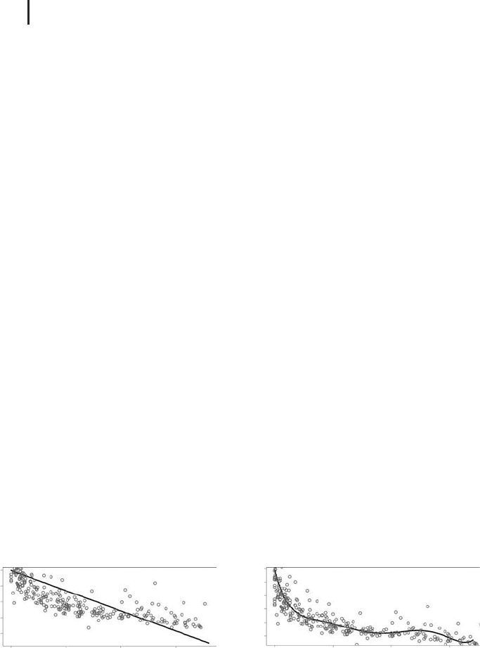
Fig. 2.3 (a) Comparison of the regression line Equation

2.39 with the data

GAG.csv.Figureproducedusing

LinRegEx4.r. (b) Comparison of the regression function

Equation 2.43 with the data

GAG.csv.Figureproducedusing

LinRegEx5.r.

2.2 Linear Regression 73

described in R as follows:

eq=GAG~Age

(2.38)

Inserting this into LinRegEx1.r (and changing the ﬁle name etc. appropriately),

one arrives at

LinRegEx4.r which you ﬁnd in the book software. Analyzing the R

output generated by

LinRegEx4.r as above, we obtain the following equation of

the regression line:

GAG(x) =−1.27 · Age + 19.89 (2.39)

Figure 2.3a compares this linear regression function with the data. As can be

seen, the regression function overestimates GAG for ages below about nine years,

and it underestimates GAG for higher ages. For ages above 15.7 years, the GAG

concentrations predicted by the regression function are negative.

This is due to the fact that the data follow some nonlinear, curved pattern which

cannot be described appropriately using a straight line. An alternative is to replace

Equation 2.27 by a polynomial regression function of the general form

y(x) = a

+ a

x + a

+···+a

(2.40)

You may wonder why such a regression function is treated here in a section

on ‘‘linear regression’’, since the function in Equation 2.40 can of course be a

highly nonlinear function of x (depending on s, the degree of the polynomial). But

remember, as was explained above in Note 2.2.1, that the term linear in ‘‘linear

regression’’ does not refer to the regression function’s dependence on x,butrather

to its dependence on the regression coefﬁcients. Seen as a function of x,Equation

2.40 certainly expresses a function that may be highly nonlinear, but if x is given,

is obtained as a linear combination of the regression coefﬁcients a

, a

, ..., a

.In

this sense, all regression functions that can be brought into the general form

y(x) = a

+ a

(x) + a

(x) +···+a

(x) (2.41)

can be treated by linear regression (where a

, a

, ..., a

are the regression coefﬁ-

cients as before, and the f

are arbitrary real functions). Whether linear or nonlinear

in x , all these functions can be treated by linear regression, and this explains the

title of this subsection (‘‘nonlinear linear regression’’).

To perform an analysis based on the polynomial regression function 2.40, we can

use R similarly as above. Basically, we just have to change the regression equation

in the previous R program

LinRegEx4.r. After some experimentation (or using

the more systematic procedure suggested in [45]) you will ﬁnd that it is a good idea

to use a polynomial of degree 6, which is written in the notation required by R

analogous to Equation 2.38 as follows:

eq=GAG~Age+I(Ageˆ2)+I(Ageˆ3)+I(Ageˆ4)+I(Ageˆ5)+I(Ageˆ6)

(2.42)

74 2 Phenomenological Models

In this equation, the R function I() is used to inhibit the interpretation of

terms like

Age^2 based on the special meaning of the ‘‘^’’ operator in R’s formula

language. Written as ‘‘

I(Age^2)’’, the ‘‘^’’ operator is interpreted as the usual

arithmetical exponentiation operator. The R program

LinRegEx5.r in the book

software uses the regression function described in Equation 2.42. Executing this

program and analyzing the results as before, the following regression function is

obtained (coefﬁcients are rounded for brevity):

GAG(x) = 29.3 − 16.2 · Age + 6 · Age

− 1.2 · Age

+0.1 · Age

− 5.7e-03 · Age

+ 1.1e-04 · Age

(2.43)

Figure 2.3b compares this regression function with the data. As can be seen,

this regression function ﬁts the data much better than the straight line that

was used in Figure 2.3a. This is also reﬂected by the fact that

LinRegEx4.r

(regression using the straight line) reports an R

value of 0.497 and 4.55 as the

mean (absolute) deviation between the data and the model, while

LinRegEx5.r

(polynomial regression) gives R

= 0.74 and a mean deviation of 2.8. Therefore the

polynomial regression obviously does a much better job in helping pediatricians to

evaluate GAG measurement data as described above. Note that beyond polynomial

regression, R offers functions for spline regression that may yield ‘‘smoother’’

regression functions based on a concatenation of low-order polynomials [45, 46].

Note 2.2.6 (Regression of large datasets) Beyond prediction, regression func-

tions can also be used as a concise way of expressing the information content of

large datasets similar to the GAG data example.

2.3

Multiple Linear Regression

In the last section, we have seen how the regression approach can be used to

predict a quantity of interest, y , depending on known values of another quantity,

x. In many cases, however, y will depend on several independent variables such

as x

, x

, ..., x

(n ∈ N). This case can be treated by the multiple (linear) regression

method. As we will see, the overall procedure is very similar to the approach

described in the last section.

2.3.1

The Multiple Linear Regression Problem

Let us begin with an example. Note that we could really take all kinds of examples

here due to the generality of the regression approach that can be used in all ﬁelds of

science and engineering. Every dataset could be used that consists of at least three

columns: two (or more) columns for the explanatory variables x

, x

, ...,andone