Velten K. Mathematical Modeling and Simulation: Introduction for Scientists and Engineers
Подождите немного. Документ загружается.

2.4 Nonlinear Regression 85
300
50
100
150
200
250
300
50
100
150
200
250
V (10
−1 Pa s)
V (10
−1 Pa s)
500
T (s)
T (s)
20
0
100
80
60
40
20
W (g)
500
400
300
200
100
0
100
60
80
40
20
W (g)
(a) (b)
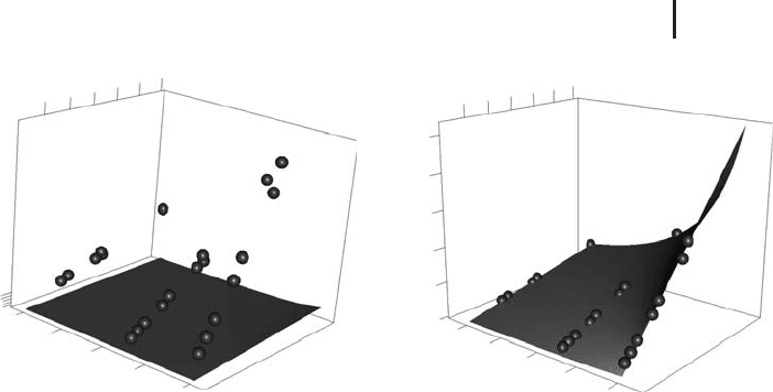
Fig. 2.7 (a) T(v, w)
according to Equation 2.58 using the
starting values a
1
= 1anda
2
= 0 (surface) compared with
the data in
stormer.csv (spheres). (b) Same plot, but us-
ing the estimates a
1
= 29.4013 and a
2
= 2.2183 obtained by
nonlinear regression using R’s
nls function. Plots generated
by
NonRegEx2.r.
need positive T values (which gives a
1
> 0 if we assume w > a
2
), and the choice
a
2
= 0 basically expresses that nothing is known about that parameter. In fact,
there is some a priori knowledge on these parameters that can be used to get more
realistic starting values (see [45]), but this example nevertheless shows that
nls
may also converge using very rough estimates of the parameters.
Figures 2.7 and 2.8 show the results produced by
NonRegEx2.r. First of all,
Figure 2.7a shows that there is substantial deviation between the regression
function Equation 2.58 and the data in
stormer.csv if the above starting values
of a
1
and a
2
are used. Figure 2.7b shows the same picture using the estimates of
a
1
and a
2
obtained by R’s nls function, and you can see by a comparison of these
two plots that the nonlinear regression procedure virtually deforms the regression
surface defined by Equation 2.58 until it fits the data. As Figure 2.7b shows, the
fit between the model and the data is almost perfect, which is also reflected by
the R
2
value computed by NonRegEx2.r (R
2
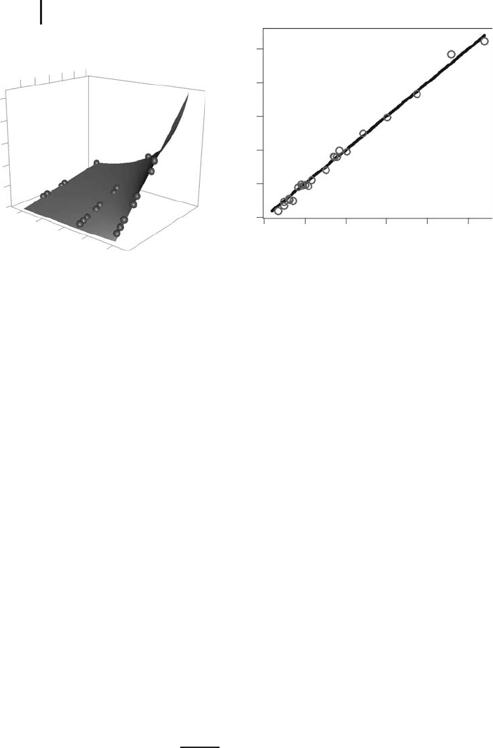
= 0.99). Figure 2.8 compares the
regression result displayed in the conventional plot that really shows the regression
function T(v, w) (Figure 2.8a) with the predicted-measured plot that was introduced
in Section 2.3 above (Figure 2.8b). The message of both plots in Figure 2.8 is the
same: an almost perfect coincidence between the regression function and the data.
Beyond this, Figure 2.8a is of course more informative compared to Figure 2.8b
since you can identify the exact location of any data point in the v/w space,
for example, the location of data points showing substantial deviations from the
regression function. Also, a plot such as Figure 2.8a allows you to assess whether
the regression function is sufficiently characterized by data, and in which regions
86 2 Phenomenological Models
300
50
100
150
200
250
V (10
−1 Pas)
500
400
300
200
100
T (s)
0
100
80
60
40
20
w (g)
250200150100500
0 50 100 150 200 250
T, predicted (s)
T, measured (s)
(a) (b)
Fig. 2.8 Comparison of the regression equation with the
data (a) in a conventional plot as in Figure 2.7 and (b) in
a predicted-measured plot. Plots generated by
NonRegEx2.r.
of the v/w space additional experimental data are needed. Looking at Figure 2.8a,
for example, the nonlinearity of the regression surface obviously is sufficiently
well characterized by the three ‘‘rows’’ of data. You should note, however, that
conventional plots such as Figure 2.8a are only available for regressions involving
up to two independent variables. Regressions involving more than two independent
variables are usually visualized using a predicted-measured plot such as Figure 2.8b,
or by using a conventional plot such as Figure 2.8a that uses two of the independent
variables of the regression and neglects the other independent variables (of course,
such conventional plots must be interpreted with care).
2.4.4
Implicit and Vector-Valued Problems
So far we have discussed two examples of nonlinear regressions referring to
regression functions of the form
ˆ
y(x) = f (x, a) (2.61)
The particular form of the regression function in the investment data example
was
f (x, a
0
, a
1
, a
2
) = a
0
· sin(a
1
· (x − a
2
)) (2.62)
In the viscometer example we had
f (x
1
, x
2
, a
1
, a
2
) =
a
1
x
1
x
2
− a
2
(2.63)

2.5 Neural Networks 87
This can be generalized in various ways. For example, the regression function
may be given implicitly as the solution of a differential equation, see the example
in Section 3.9.
ˆ
y may also be a vector-valued function
ˆ
y = (
ˆ
y
1
, ...,
ˆ
y
r
). An example
of this kind will be discussed below in Section 3.10.2. The nonlinear regression
function then takes the form
ˆ
y(x) = f (x, a) (2.64)
where x = (x
1
, ..., x
n
) ∈ R
n
, a = (a
1
, ..., a
s
) ∈ R
s
,and
ˆ
y(x)andf (x, a) are real vector
functions
ˆ
y(x) = (
ˆ
y
1
(x), ...,
ˆ
y
r
(x)), f (x, a) = (f
1
(x, a), ..., f
r
(x, a)) (r, s, n ∈ N).
2.5
Neural Networks
If we perform a nonlinear regression analysis as described above, we need to know
the explicit form of the regression function. In our analysis of the investment data
klein.csv, the form of the regression function (a sine function) was derived from
the sinusoidal form of the data in a graphical plot. In some cases, we may know
an appropriate form of the regression function based on a theoretical reasoning, as
was the case in our above analysis of the stormer viscometer data
stormer.csv.
But there are, of course, situations where the type of regression function cannot
be derived from theory, and where graphical plots of the data are unavailable (e.g.
because there are more than two independent variables). In such cases, we can try
for example, polynomial or spline regressions (see the example in Section 2.2), or
so-called (artificial) neural networks (ANN).
Note 2.5.1 (Application to regression problems) Among other applications (see
below), neural networks can be used as particularly flexible nonlinear regression
functions. They provide a great number of tuning parameters that can be used to
approximate any smooth function.
2.5.1
General Idea
To explain the idea, let us reconsider the multiple linear regression function
ˆ
y = a
0
+ a
1
x
1
+ a
2
x
2
+···+a
n
x
n
(2.65)
Aswasdiscussedabove,thisequationisablackbox–typemodelofan
input–output system (Figure 1.2), where x
1
, ..., x
n
are the given input quanti-
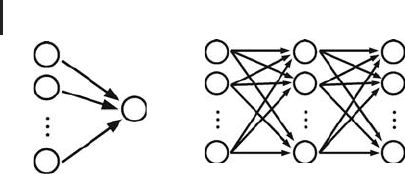
ties and y is the output quantity computed from the inputs. Graphically, this can be
interpreted as shown in Figure 2.9a. The figure shows a network of nodes where each
of the nodes corresponds to one of the quantities x
1
, ..., x
n
and y. The nodes are
88 2 Phenomenological Models
OutputInput
Input
layer
Hidden
layer
Output
layer
x
1
x
1
y
1
y
2
y
m
x
2
x
2
x
n
x
n
y
(a) (b)
Fig. 2.9 (a) Graphical interpretation of multiple regression.
(b) Artificial neural network with one hidden layer.
grouped together into one layer comprising the input nodes x
1
, ..., x
n
,andasecond
layer comprising the output node y. The arrows indicate that the information flow
is from the input nodes toward the output node, similar to Figure 1.2 above. Now
the multiple linear regression equation (2.65) can be viewed as expressing the way
in which the output node processes the information that it gets from the input
nodes: each of the input node levels x
1
, ..., x
n
is multiplied with a corresponding
constant a
1
, ..., a
n
, the results are added up, and the level of the output node y is
then obtained as this sum plus a constant (the so-called bias) a
0
.
So far, this is no more than a graphical interpretation of multiple regression.
This interpretation becomes interesting in view of its analogy with neural networks
in biological tissues such as the human brain. Formally, such neural networks
can also be described by figures similar to Figure 2.9a, that is, as a system of
interconnected nodes (corresponding to the biological neurons) which exchange
information along their connections [53, 54]. Since the information exchange in
biological neural networks is of great importance if one e.g. wants to understand
the functioning of the human brain, a great deal of research has been devoted
to this topic in the past. As a part of this research effort, mathematical models
have been developed that describe the information exchange in interconnected
networks such as the network shown in Figure 2.9a, but of course involving
more complex network topologies than the one shown in Figure 2.9a, and more
complex (nonlinear) equations than the simple multiple linear regression equation,
Equation 2.65.
It turned out that these mathematical models of interconnected networks of
nodes are useful for their own sake, that is, independently of their biological
interpretation, e.g. as a flexible regression approach that is apt to approximate
any given smooth function. This class of mathematical models of interconnected
networks of nodes are called (artificial) neural network models or ANN models,or
simply neural networks. They may be applied in their original biological context, or in
a great number of entirely different applications such as general regression analysis
(e.g. prediction of tribological properties of materials [55–60], or the permeability
prediction example below), time series prediction (stock prediction etc.), classification

2.5 Neural Networks 89
and pattern recognition (face identification, text recognition, etc.), data processing
(knowledge discovery in databases, e-mail spam filtering, etc.) [53, 54].
Note 2.5.2 (Analogy with biology) Multiple linear regression can be interpreted
as expressing the processing of information in a network of nodes (Figure 2.9a).
Neural networks arise from a generalization of this interpretation, involving
additional layer(s) of nodes and nonlinear operations (Figure 2.9b). Models of
this kind are called (artificial) neural networks (ANN’s) since they have been used
to describe the information processing in biological neural networks such as the
human brain.
2.5.2
Feed-Forward Neural Networks
The diversity of neural network applications corresponds to a great number of
different mathematical formulations of neural network models, and to a great
number of more or less complex network topologies used by these models [53, 54].
We will confine ourselves to the simple network topology shown in Figure 2.9b.
This network involves an input and an output layer similar to Figure 2.9a, and in
addition to this there is a so-called hidden layer between the input and output layers.
As indicated by the arrows, the information is assumed to travel from left to right
only, which is why this network type is called a feedforward neural network .Thisis
one of the most commonly used neural network architectures, and based on the
mathematical interpretation that will be given now (using ideas and notation from
[45]) it is already sufficiently complex e.g. to approximate arbitrary smooth functions.
Let us assume that there are n ∈ N input nodes corresponding to the given input
quantities x
1
, ..., x
n
, H ∈ N hidden nodes and m ∈ N output nodes corresponding
to the output quantities y
1
, ..., y
m
. Looking at the top node in the hidden layer of
Figure 2.9b, you see that this node receives its input from all nodes of the input
layer very similar to Figure 2.9a. Let us assume that this node performs the same
operation on its input as was discussed above referring to Figure 2.9a, multiplying
each of the inputs with a constant, taking the sum over all the inputs and then
adding a constant. This leads to an expression of the form
n
k=1
w
ik;h1
x
k
+ b
h1
(2.66)
Here, the so-called weight w
ik;h1
denotes the real coefficient used by the hidden
node 1 (index h1) to multiply the kth input (index ik), and b
h1
is the bias added
by hidden node 1. Apart from notation, this corresponds exactly to the multiple
linear regression equation 2.65 discussed above. The network would thus be no
more than a complex way to express multiple (linear) regression if all nodes in the

90 2 Phenomenological Models
network would do no more than the arithmetics described by Equation 2.66. Since
this would make no sense, the hidden node 1 will apply a nonlinear real function
φ
h
to Equation 2.66, giving
φ
h
n
k=1
w
ik;h1
x
k
+ b
h1
(2.67)
The application of this so-called activation function is the basic trick that really acti-
vates the network and makes it a powerful instrument far beyond the scope of linear
regression. The typical choice for the activation function is the logistic function
f (x) =
e
x
1 +e
x
(2.68)
The state of the hidden nodes l = 1, ..., H after the processing of the inputs can
be summarized as follows:
φ
h
n
k=1
w
ik;hl
x
k
+ b
hl
, l = 1, ..., H (2.69)
These numbers now serve as the input of the output layer of the network.
Assuming that the output layer processes this input the same way as the hidden
layer based on different coefficients and a different nonlinear function φ
o
,the
output values are obtained as follows:
y
j
= φ
o
b
oj
+
H
l=1
w
hl,oj
· φ
h
b
hl
+
n
k=1
w
ik;hl
· x
k
, j = 1, ..., m (2.70)
Similar as above, the weights w
hl,oj
denote the real coefficient used by the output
node j (index oj) to multiply the input from the hidden node l (index hl), and b
oj
is the bias added by output node j.Below,wewillusR’s nnet command to fit
this equation to data. This command is restricted to single-hidden-layer neural
networks such as the one shown in Figure 2.9b.
nnet nevertheless is a powerful
command since the following can be shown [45, 61–63]:
Note 2.5.3 (Approximation property) The single-hidden-layer feedforward neu-
ral network described in Equation 2.70 can approximate any continuous function
f : ⊂ R
n
→ R
m
uniformly on compact sets by increasing the size of the hidden
layer (if linear output units φ
o
are used).
The
nnet command is able to treat a slightly generalized version of Equation
2.70 which includes so-called skip-layer connections:
y
j
= φ
o
b
oj
+
n
k=1
w
ik;oj
· x
k
+
H
l=1
w
hl,oj
· φ
h
b
hl
+
n
k=1
w
ik;hl
· x
k
, (2.71)
j = 1, ..., m

2.5 Neural Networks 91
Referring to the network topology in Figure 2.9b, skip-layer connections are
direct connections from each of the input units to each of the ouput units, that
is, connections which skip the hidden layer. Since you can probably imagine how
Figure 2.9b will look after adding these skip-layer connections, you will understand
why we skip this here... As explained in [45], the important point is that skip layer
connections make the neural network more flexible, allowing it to construct the
regression surface as a perturbation of a linear hyperplane (again, if φ
o
is linear). In
Equation 2.71, the skip layer connections appear in the terms w
ik;oj
· x
k
,whichisthe
result of input node k after processing by the output node j. Again, the weights w
ik;oj
are real coefficients used by the output nodes to multiply the numbers received by
the input nodes along the skip-layer connections.
Similar to above, Equation 2.71 can be fitted to data by a minimization of RSQ
(similar to the discussion in Section 2.2.1, see also [45] for alternative optimization
criteria provided by the
nnet command that will be treated in Section 2.5.3 below).
Altogether, the number of weights and biases appearing in Equation 2.71 is
N
p
= H(n + 1) + mH + mn + 1 (2.72)
So you see that there is indeed a great number of ‘‘tuning’’ parameters that can be
used to achieve a good fit between the model and the data, which makes it plausible
that a statement such as Note 2.5.3 can be proved.
2.5.3
Solution Using Software
As a first example, let us look at Klein’s investment data again (klein.csv,see
Section 2.4). Above, a sine function was fitted to the data, leading to a residual sum
of squares of RSQ = 105.23 (Figure 2.6). Let us see how a neural network performs
on these data. An appropriate Rprogramis
NNEx1.r, which you find in the book
software. Basically,
NNEx1.r is obtained by just a little editing of NonRegEx1.r
that was used in Section 2.4 above: we have to replace the nonlinear regression
command
nls used in NonRegEx1.r by the nnet command that computes the
neural network. Let us look at the part of
NNEx1.r that does the neural network
computing:
1: eq=inv~year
2: FileName="Klein.csv"
3: Data=read.table(FileName,
...)
4: Scaled=data.frame(year=Data$year/1941,inv=Data$inv)
5: NNModel=nnet(eq,data=Scaled,size=3,decay=1e-4,
5: linout=T, skip=T, maxit=1000, Hess=T)
6: eigen(NNModel$Hessian)$values
(2.73)
In line 1, year and inv are specified as the input and output quantities of the
model, respectively. Note that in contrast to our last treatment of these data in

92 2 Phenomenological Models
Section 2.4, we do not need to specify the nonlinear functional form of the data
which will be detected automatically by the neural network (compare line 1 of
program 2.73 with line 1 of program 2.57). After the data have been read in lines
2and3,theexplanatoryvariable
year (which ranges between 1920 and 1941) in
Klein.csv is rescaled to a range between 0 and 1, which is necessary for the
reasons explained in [45]. A little care is necessary to distinguish between scaled
and unscaled data particularly in the plotting part of the code (see
NNEx1.r).
Note 2.5.4 (R’s nnet command) In R,thennet command can be used
to compute a single-hidden layer feedforward neural network (Equation 2.71).
Before using this command, the input data should be scaled to a range between
0and1.
The neural network model
NNModel is obtained in line 5 using R’s nnet
command. nnet uses the equation eq from line 1 and the scaled data Scaled
from line 4. Beyond this, the size argument determines the number of nodes
in the hidden layer; the
decay argument penalizes overfitting, which will be
discussed below;
linout=T defines linear activation functions for the output units
(i.e. φ
o
is linear); skip=T allows skip-layer connections; maxit=1000 restricts the
maximum number of iterations of the numerical procedure, and
Hess=T instructs
nls to compute the Hessian matrix which can be used to check if a secure local
minimum was achieved by the algorithm (see below). Note that
linout and skip
are so-called logical variables which have the possible values ‘‘T’’ (true) or ‘‘F’’ (false).
Line 6 of the code is again related to the Hessian matrix and will be discussed
below.
2.5.4
Interpretation of the Results
When you execute NNEx1.r in R,thennet command will determine the parameters
of Equation 2.71 such that the y
j
computed by Equation 2.71 lie close to the data
klein.csv, by default in the sense of a minimal RSQ as explained above.
Remember that there are two kinds of parameters in Equation 2.71: the weights
w
ik;oj
, w
hl,oj
,andw
ik;hl
which are used by the nodes of the network to multiply their
input values, and the biases b
oj
and b
hl
which are added to the weighted sums
of the values of the hidden layer or of the input layer.
NNEx1.r uses a network
with 3 nodes in the hidden layer (line 5 of program 2.73), which means that in
Equation 2.71 we have n = 1, H = 3andm = 1. Using Equation 2.72, you see that
this gives a total number of N
p
= 11 parameters that must be determined by nnet.
Since Equation 2.71 is nonlinear, these parameters are determined by an iterative
numerical procedure similar to the one discussed in Section 2.4 above [45, 64].
This procedure needs starting values as discussed above. In some cases, you may
know appropriate starting values, which can be supplied to
nnet in a way similar
to the one used above for the
nls command (see Section 2.4 and R’s help pages on
2.5 Neural Networks 93
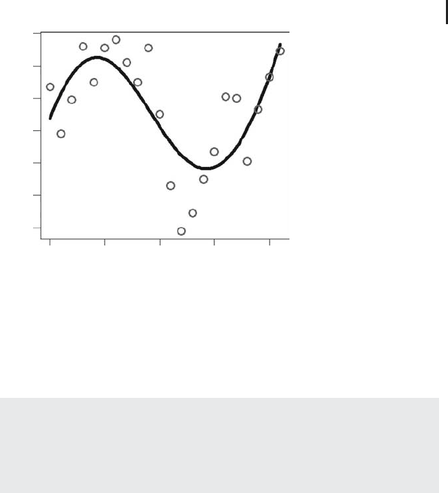
6
4
2
0
−2
−4
−6
1920 1925 1930 1935 1940
Year
I
Fig. 2.10 Comparison of the neural network Equation
2.71 based on the parameters in program 2.73 (line) with
the data in
klein.csv (circles). Figure produced using
NNEx1.r.
the nnet command). If you do not specify those starting values yourself, the nnet
command uses automatically generated random numbers as starting values.
Note 2.5.5 (Random choice of starting values) Similar to the nls command
that can be used for nonlinear regression (see Section 2.4), R’s
nnet command
fits a neural network to data using an iterative procedure. By default, the starting
values for the network weights and biases are chosen randomly, which implies
that the results of subsequent runs of
nnet will typically differ.
Executing
NNEx1.r several times, you will see that some of the results will be
unsatisfactory (similar to a mere linear regression through the data), while other
runs will produce a picture similar to Figure 2.10. This figure is based on the
skip-layer neural network equation 2.71 using the following parameters:
b->h1 i1->h1
124.29 -125.32
b->h2 i1->h2
357.86 -360.13
b->h3 i1 ->h3
106.45 -107.35
b->o h1->o h2->o h3->o i1->o
41.06 -195.48 136.35 -156.09 48.32
(2.74)
An output similar to 2.74 is a part of the results produced by nnet.The
correspondence with the parameters of Equation 2.71 is obvious: for example,

94 2 Phenomenological Models
‘‘b->h1’’ refers to the bias added by the hidden layer node 1, which is b
h1
in the
notation of Equation 2.71, and hence 2.74 tells us that b
h1
= 124.29. ‘‘i1->h1’’
refers to the weight used by the hidden layer node 1 to multiply the value of input
node 1, which is w
i1;h1
in the notation of Equation 2.71, and hence 2.74 tells us that
w
i1;h1
=−125.32. Note that ‘‘i1->o’’ is the weight of the skip-layer connection
(i.e. we have w
i1;o1
= 48.32).
Note that the results in Figure 2.10 are very similar to the results obtained above
using a sinusoidal nonlinear regression function (Figure 2.6). The difference is
that in this case the sinusoidal pattern in the data was correctly found by the neural
network without the need to find an appropriate expression of the regression
function before the analysis is performed (e.g. based on a graphical analysis of the
data as above). As explained above, this is particularly relevant in situations where
it is hard to get an appropriate expression of the regression function, for example,
when we are concerned with more than two input quantities where graphical plots
involving the response variable and all input quantities are unavailable. The RSQ
produced by the network shown in Figure 2.10 (RSQ = 103.41) is slightly better
than the one obtained for the nonlinear regression function in Figure 2.6 (RSQ
= 105.23). Comparing these two figures in detail, you will note that the shape
of the neural network in Figure 2.10 is not exactly sinusoidal: its values around
1940 exceed its maximum values around 1925. This underlines the fact that neural
networks are governed by the data only (if sufficient nodes in the hidden layer are
used): the neural network in Figure 2.10 describes an almost sinusoidal shape,
but it also detects small deviations from a sinusoidal shape. In this sense, neural
networks have the potential to perform better compared to nonlinear regression
functions such as the one used in Figure 2.6 which is restricted to an exact
sinusoidal shape.
Note 2.5.6 (Automatic detection of nonlinearities) Neural networks describe
the nonlinear dependency of the response variable on the explanatory variables
without a previous explicit specification of this nonlinear dependency (which is
required in nonlinear regression, see Section 2.4).
The
nnet command determines the parameters of the network by a minimization
of an appropriate fitting criterion [45, 64]. Using the default settings, the RSQ will be
used in a way similar to the above discussion in Sections 2.2 and 2.4. The numerical
algorithm that works inside
nnet thus minimizes e.g. RSQ as a function of the
parameters of the neural network, Equation 2.71, that is, as a function of the weights
w
ik;oj
, w
hl,oj
, w
ik;hl
and of the biases b
oj
and b
hl
. Formally, this is the minimization of
a function of several variables, and you know from calculus that if a particular value
of the independent variable is a local minimum of such a function, the Hessian
matrix at that point is positive definite, which means that the eigenvalues of the
Hessian matrix at that point are positive [65]. In line 6 of 2.73, the eigenvalues of
the Hessian matrix are computed (referring to the particular weights and biases
found by
nnet), and the result corresponding to the neural network in Figure 2.10